4. Query Language Guide
4.1. Preface
4.1.1. Overview
This guide provides information about how to use the rasdaman database management system (in short: rasdaman). The document explains usage of the rasdaman Query Language.
Follow the instructions in this guide as you develop your application which makes use of rasdaman services. Explanations detail how to create type definitions and instances; how to retrieve information from databases; how to insert, manipulate, and delete data within databases.
4.1.2. Audience
The information in this manual is intended primarily for application developers; additionally, it can be useful for advanced users of rasdaman applications and for database administrators.
4.1.3. Rasdaman Documentation Set
This manual should be read in conjunction with the complete rasdaman documentation set which this guide is part of. The documentation set in its completeness covers all important information needed to work with the rasdaman system, such as programming and query access to databases, guidance to utilities such as raswct, release notes, and additional information on the rasdaman wiki.
4.2. Introduction
4.2.1. Multidimensional Data
In principle, any natural phenomenon becomes spatio-temporal array data of some specific dimensionality once it is sampled and quantised for storage and manipulation in a computer system; additionally, a variety of artificial sources such as simulators, image renderers, and data warehouse population tools generate array data. The common characteristic they all share is that a large set of large multidimensional arrays has to be maintained. We call such arrays multidimensional discrete data (or short: MDD) expressing the variety of dimensions and separating them from the conceptually different multidimensional vectorial data appearing in geo databases.
rasdaman is a domain-independent database management system (DBMS) which supports multidimensional arrays of any size and dimension and over freely definable cell types. Versatile interfaces allow rapid application deployment while a set of cutting-edge intelligent optimization techniques in the rasdaman server ensures fast, efficient access to large data sets, particularly in networked environments.
4.2.2. Rasdaman Overall Architecture
The rasdaman client/server DBMS has been designed using internationally approved standards wherever possible. The system follows a two-tier client/server architecture with query processing completely done in the server. Internally and invisible to the application, arrays are decomposed into smaller units which are maintained in a conventional DBMS, for our purposes called the base DBMS.
On the other hand, the base DBMS usually will hold alphanumeric data (such as metadata) besides the array data. Rasdaman offers means to establish references between arrays and alphanumeric data in both directions.
Hence, all multidimensional data go into the same physical database as the alphanumeric data, thereby considerably easing database maintenance (consistency, backup, etc.).
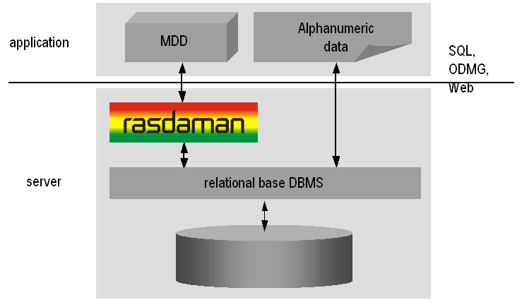
Figure 4.1 Embedding of rasdaman in IT infrastructure
Further information on application program interfacing, administration, and related topics is available in the other components of the rasdaman documentation set.
4.2.3. Interfaces
The syntactical elements explained in this document comprise the rasql language interface to rasdaman. There are several ways to actually enter such statements into the rasdaman system:
By using the rasql command-line tool to send queries to rasdaman and get back the results.
By developing an application program which uses the raslib/rasj function
oql_execute()to forward query strings to the rasdaman server and get back the results.
Developing applications using the client API is the subject of this document. Please refer to the C++ Developers Guide or Java Developers Guide of the rasdaman documentation set for further information.
4.2.4. rasql and Standard SQL
The declarative interface to the rasdaman system consists of the rasdaman Query Language, rasql, which supports retrieval, manipulation, and data definition.
Moreover, the rasdaman query language, rasql, is very similar - and in fact embeds into - standard SQL. With only slight adaptations, rasql has been standardized by ISO as 9075 SQL Part 15: MDA (Multi-Dimensional Arrays). Hence, if you are familiar with SQL, you will quickly be able to use rasql. Otherwise you may want to consult the introductory literature referenced at the end of this chapter.
4.2.5. Notational Conventions
The following notational conventions are used in this manual:
Program text (under this we also subsume queries in the document on hand) is
printed in a monotype font. Such text is further differentiated into
keywords and syntactic variables. Keywords like struct are printed in boldface;
they have to be typed in as is.
An optional clause is enclosed in brackets; an arbitrary repetition is indicated
through brackets and an asterisk. Grammar alternatives can be grouped in
parentheses separated by a | symbol.
Example
selectresultListfromcollName[ [ as ]collAlias] [ ,collName[ [ as ]collAlias] ]* [ wherebooleanExp]
It is important not to mix the regular brackets [ and ] denoting array
access, trimming, etc., with the grammar brackets [ and ] denoting
optional clauses and repetition; in grammar excerpts the first case is in
double quotes. The same applies to parentheses.
Italics are used in the text to draw attention to the first instance of a defined term in the text. In this case, the font is the same as in the running text, not Courier as in code pieces.
4.3. Terminology
4.3.1. An Intuitive Definition
An array is a set of elements which are ordered in space. The space considered here is discretized, i.e., only integer coordinates are admitted. The number of integers needed to identify a particular position in this space is called the dimension (sometimes also referred to as dimensionality). Each array element, which is referred to as cell, is positioned in space through its coordinates.
A cell can contain a single value (such as an intensity value in case of grayscale images) or a composite value (such as integer triples for the red, green, and blue component of a color image). All cells share the same structure which is referred to as the array cell type or array base type.
Implicitly a neighborhood is defined among cells through their coordinates: incrementing or decrementing any component of a coordinate will lead to another point in space. However, not all points of this (infinite) space will actually house a cell. For each dimension, there is a lower and upper bound, and only within these limits array cells are allowed; we call this area the spatial domain of an array. In the end, arrays look like multidimensional rectangles with limits parallel to the coordinate axes. The database developer defines both spatial domain and cell type in the array type definition. Not all bounds have to be fixed during type definition time, though: It is possible to leave bounds open so that the array can dynamically grow and shrink over its lifetime.
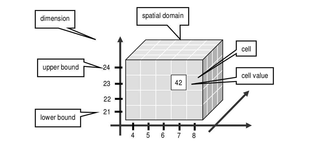
Figure 4.2 Constituents of an array
Synonyms for the term array are multidimensional array / MDA, multidimensional data / MDD, raster data, gridded data. They are used interchangeably in the rasdaman documentation.
In rasdaman databases, arrays are grouped into collections. All elements of a collection share the same array type definition (for the remaining degrees of freedom see Array types). Collections form the basis for array handling, just as tables do in relational database technology.
4.3.2. A Technical Definition
Programmers who are familiar with the concept of arrays in programming languages maybe prefer this more technical definition:
An array is a mapping from integer coordinates, the spatial domain, to some data type, the cell type. An array’s spatial domain, which is always finite, is described by a pair of lower bounds and upper bounds for each dimension, resp. Arrays, therefore, always cover a finite, axis-parallel subset of Euclidean space.
Cell types can be any of the base types and composite types defined in the ODMG standard and known, for example from C/C++. In fact, most admissible C/C++ types are admissible in the rasdaman type system, too.
In rasdaman, arrays are strictly typed wrt. spatial domain and cell type. Type checking is done at query evaluation time. Type checking can be disabled selectively for an arbitrary number of lower and upper bounds of an array, thereby allowing for arrays whose spatial domains vary over the array lifetime.
4.4. Sample Database
4.4.1. Collection mr
This section introduces sample collections used later in this manual. The sample database which is shipped together with the system contains the schema and the instances outlined in the sequel.
Collection mr consists of three images (see Figure 4.3) taken from the
same patient using magnetic resonance tomography. Images are 8 bit
grayscale with pixel values between 0 and 255 and a size of 256x211.
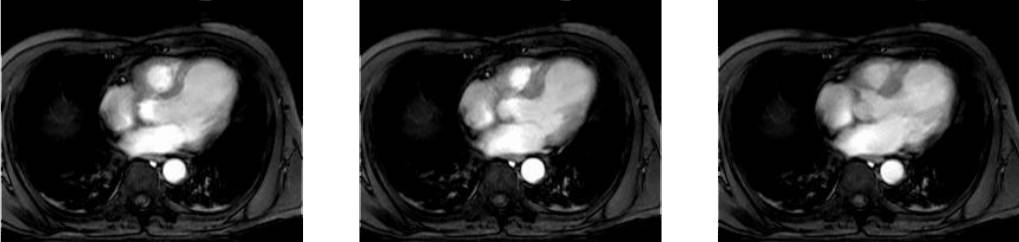
Figure 4.3 Sample collection mr
4.4.2. Collection mr2
Collection mr2 consists of only one image, namely the first image of
collection mr (Figure 4.4). Hence, it is also 8 bit grayscale with
size 256x211.
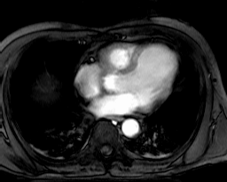
Figure 4.4 Sample collection mr2
4.4.3. Collection rgb
The last example collection, rgb, contains one item, a picture of the
anthur flower (Figure 4.5). It is an RGB image of size 400x344 where
each pixel is composed of three 8 bit integer components for the red, green, and
blue component, resp.

Figure 4.5 The collection rgb
4.5. Type Definition Using rasql
4.5.1. Overview
Every instance within a database is described by its data type (i.e., there is exactly one data type to which an instance belongs; conversely, one data type can serve to describe an arbitrary number of instances). Each database contains a self-contained set of such type definitions; no other type information, external to a database, is needed for database access.
Types in rasdaman establish a 3-level hierarchy:
Cell types can be atomic base types (such as char or float) or composite (“struct”) types such as red / green / blue color pixels.
Array types define arrays over some atomic or struct cell type and a spatial domain.
Set types describe sets of arrays of some particular array type.
Types are identified by their name which must be unique within a database and not exceed length of 200 characters. Like any other identifier in rasql queries, type names are case-sensitive, consist of only letters, digits, or underscore, and must start with a letter.
4.5.2. Cell types
4.5.2.1. Atomic types
The set of standard atomic types, which is generated during creation of a database, materializes the base types defined in the ODMG standard (cf. Table 4.1).
type name |
size |
description |
|---|---|---|
|
1 bit [2] |
true (nonzero value), false (zero value) |
|
8 bit |
signed integer |
|
8 bit |
unsigned integer |
|
16 bit |
signed integer |
|
16 bit |
unsigned integer |
|
32 bit |
signed integer |
|
32 bit |
unsigned integer |
|
32 bit |
single precision floating point |
|
64 bit |
double precision floating point |
|
32 bit |
complex of 16 bit signed integers |
|
64 bit |
complex of 32 bit signed integers |
|
64 bit |
single precision floating point complex |
|
128 bit |
double precision floating point complex |
4.5.2.2. Composite types
More complex, composite cell types can be defined arbitrarily, based on the system-defined atomic types. The syntax is as follows:
create type typeName
as (
  attrName_1 atomicType_1,
  ...
  attrName_n atomicType_n
)
Attribute names must be unique within a composite type, otherwise an
exception is thrown. No other type with the name typeName may pre-exist
already.
4.5.2.3. Example
An RGB pixel type can be defined as
create type RGBPixel
as (
  red char,
  green char,
  blue char
)
4.5.3. Array types
An marray (“multidimensional array”) type defines an array type through its cell type (see Cell types) and a spatial domain.
4.5.3.1. Syntax
The syntax for creating an marray type is as below. There are two variants, corresponding to the dimensionality specification alternatives described above:
create type typeName
as baseTypeName mdarray namedMintervalExp
where baseTypeName is the name of a defined cell type (atomic or composite)
and namedMintervalExp is a multidimensional interval specification as described
in the following section.
Alternatively, a composite cell type can be indicated in-place:
create type typeName
as (
  attrName_1 atomicType_1,
  ...
  attrName_n atomicType_n
) mdarray namedMintervalExp
No type (of any kind) with name typeName may pre-exist already,
otherwise an exception is thrown.
Attribute names must be unique within a composite type, otherwise an exception is thrown.
4.5.3.2. Spatial domain
Dimensions and their extents are specified by providing an axis name for each dimension and, optionally, a lower and upper bound:
[ a_1 ( lo_1 : hi_1 ), ... , a_d ( lo_d : hi_d ) ]

[ a_1 , ... , a_d ]
where d is a positive integer number, a_i are identifiers, and lo_1
and hi_1 are integers such that lo_1 \(\le\) hi_1. Both lo_1
and hi_1 can be an asterisk (*) instead of a number, in which case no
limit in the particular direction of the axis will be enforced. If the bounds
lo_1 and hi_1 on a particular axis are not specified, they are assumed
to be equivalent to *.
Axis names must be unique within a domain specification, otherwise an exception is thrown.
Currently axis names are ignored and cannot be used in queries yet.
4.5.3.3. Examples
The following statement defines a 2-D RGB image, based on the definition of
RGBPixel as shown above:
create type RGBImage
as RGBPixel mdarray [ x ( 0:1023 ), y ( 0:767 ) ]
An 2-D image without any extent limitation can be defined through:
create type UnboundedImage
as RGBPixel mdarray [ x, y ]
which is equivalent to
create type UnboundedImage
as RGBPixel mdarray [ x ( *:* ), y ( *:* ) ]
Selectively we can also limit only the bounds on the x axis for example:
create type PartiallyBoundedImage
as RGBPixel mdarray [ x ( 0 : 1023 ), y ]
4.5.4. Set types
A set type defines a collection of arrays sharing the same marray type. Additionally, it can indicate that some cell values in these arrays are null. Null is a special marker commonly used in databases to indicate non-existing data values. In rasdaman, it means that in some array cell there is no value that can be used for anything. A variety of reasons exist for such missing values: a sensor detected an erroneous reading, no value was provided at all (maybe due to transmission problems), no values are applicable to this position at all (such as sea surface temperature measurements on dry land positions), etc. As arrays by definition have a value for every position inside the array spatial domain, a “placeholder” must exist which reserves the place (thereby not disturbing array order) while indicating that the value is not to be used. We call such cells null values.
In rasdaman two ways exist to model null values:
by keeping a flag (called “null flag” or “null mask”) for each cell indicating whether it is null or not; this is the common approach in databases;
by designating one or more of the possible values of a cell as representing a null value; we call the set of these possible values the “null set”; this is the common way of representing nulls in sensor data acquisition.
Starting with version 10.0 both methods are supported by rasdaman in a compatible manner. The null set is important for compatibility with sensor data encoded in various formats, while the null mask is crucial for producing accurate results during query processing.
This section explains how to specify null values in the array set definition. Dynamically setting null set and mask in an expression and null behavior in operations is explained in Null Values.
4.5.4.1. Syntax
createSetType:
  create type setTypeName
  as set '(' marrayTypeName (nullClause)? ')'

nullClause:
  null values nullSet
| null values { nullSet, nullSet* }

nullSet: [ nullSetMember, nullSetMember* ]

nullSetMember:
  number : number
|    "*" : number
| number : "*"
| number
where marrayTypeName is the name of a defined marray type and nullClause
is an optional specification of a set of values to be treated as nulls.
No type with the name setTypeName may pre-exist already.
4.5.4.2. Semantics
The optional nullClause allows associating N null sets with the created set
type. Let B be the base type of marrayTypeName. The number of null sets N
can be
1, in which case the single null set applies to each band of B
K, where K is the number of bands defined by the composite type B; in this case the K null sets are enclosed in braces
Any other case results in an error.
A cell value of an array band is a null value if it matches any of the
nullSetMember in the null set defined by the nullClause. Each
nullSetMember expression is matched as follows depending on the syntax used:
lo:hi- any value between and inclusive lo and hi is a null value; lo and hi are numbers such that lo ≤ hi, and conform to the base type defined by the set type;*:hi- any value lower than or equal to hi is a null value;lo:*- any value greater than or equal to lo is a null value;x- any value equal to x is a null value. For floating-point data it is recommended to always specify sufficiently large intervals to include neighboring numbers generated through rounding errors, instead of single numbers with this variant.For floating-point base type, x can additionally be set to NaN with
nanfor base type double, andnanffor base type float.
All lo, hi, and x in the null set must be within the range of values supported
by the base type of marrayTypeName, e.g. 0 to 255 for base type char;
otherwise a type error will be thrown.
4.5.4.3. Examples
The following statement defines a set type of 2-D RGB images, based on the
definition of RGBImage:
create type RGBSet
as set ( RGBImage )
If values 0, 253, 254, and 255 are to be considered null values, this can be specified as follows:
create type RGBSet
as set ( RGBImage null values [ 0, 253 : 255 ] )
Note that these null values will apply equally to every band.
As the cell type in this case is char (possible values between 0 and 255), the type can be equivalently specified like this:
create type RGBSet
as set ( RGBImage null values [ 0, 253 : * ] )
In the first band values equal to 0 are null values, while in the second and third bands null values are those equal to 255:
create type RGBSetSeparateNullValues
as set ( RGBImage null values { [0], [255], [255] } )
With the set type below, values which are nan are null values (nanf is the float constant, while nan is the double constant):
create type FloatSetNanNullValue
as set ( FloatImage null values [nanf] )

create type DoubleSetNanNullValue
as set ( DoubleImage null values [nan] )
4.5.5. Drop type
A type definition can be dropped (i.e., deleted from the database) if it is not in use. This is the case if both of the following conditions hold:
The type is not used in any other type definition.
There are no array instances existing which are based, directly or indirectly, on the type on hand.
Further, atomic base types (such as char) cannot be deleted.
Drop type syntax
drop type typeName
4.5.6. List available types
A list of all types defined in the database can be obtained in textual
form, adhering to the rasql type definition syntax. This is done by
querying virtual collections (similar to the virtual collection
RAS_COLLECTIONNAMES).
Technically, the output of such a query is a list of 1-D char arrays,
each one containing one type definition.
4.5.6.1. Syntax
select typeColl from typeColl
where typeColl is one of
RAS_STRUCT_TYPESfor struct typesRAS_MARRAY_TYPESfor array typesRAS_SET_TYPESfor set typesRAS_TYPESfor union of all types
Note
Collection aliases can be used, such as:
select t from RAS_STRUCT_TYPES as t
No operations can be performed on the output array.
4.5.6.2. Example output
A struct types result may look like this when printed:
create type RGBPixel
as ( red char, green char, blue char )

create type TestPixel
as ( band1 char, band2 char, band3 char )

create type GeostatPredictionPixel
as ( prediction float, variance float )
An marray types result may look like this when printed:
create type GreyImage
as char mdarray [ x, y ]

create type RGBCube
as RGBPixel mdarray [ x, y, z ]

create type XGAImage
as RGBPixel mdarray [ x ( 0 : 1023 ), y ( 0 : 767 ) ]
A set types result may look like this when printed:
create type GreySet
as set ( GreyImage )

create type NullValueTestSet
as set ( NullValueArrayTest null values [5:7] )
An all types result will print combination of all struct types, marray types, and set types results.
4.5.7. Changing types
The type of an existing collection can be changed to another type through
the alter statement.
The new collection type must be compatible with the old one, which means:
same cell type
same dimensionality
no domain shrinking
Changes are allowed, for example, in the null values.
Alter type syntax
alter collection collName
set type collType
where
collName is the name of an existing collection
collType is the name of an existing collection type
Usage notes
The collection does not need to be empty, i.e. it may contain array objects.
Currently, only set (i.e., collection) types can be modified.
Example
Update the set type of a collection Bathymetry to a new set type that
specifies null values:
alter collection Bathymetry
set type BathymetryWithNullValues
4.6. Query Execution with rasql
The rasdaman toolkit offers essentially a couple of ways to communicate with a database through queries:
By submitting queries via command line using rasql; this tool is covered in this section.
By writing a C++, Java, or Python application that uses the rasdaman APIs (raslib, rasj, or rasdapy3 respectively). See the rasdaman API guides for further details.
The rasql tool accepts a query string (which can be parametrised as explained in the API guides), sends it to the server for evaluation, and receives the result set. Results can be displayed in alphanumeric mode, or they can be stored in files.
4.6.1. Examples
For the user who is familiar with command line tools in general and the rasql query language, we give a brief introduction by way of examples. They outline the basic principles through common tasks.
Create a collection
testof typeGreySet(note the explicit setting of userrasadmin; rasql’s default userrasguestby default cannot write):rasql -q "create collection test GreySet" \ --user rasadmin --passwd rasadmin
Print the names of all existing collections:
rasql -q "select r from RAS_COLLECTIONNAMES as r" \
      --out string
Export demo collection
mrinto TIFF files rasql_1.tif, rasql_2.tif, rasql_3.tif (note the escaped double-quotes as required by shell):rasql -q "select encode(m, \"tiff\") from mr as m" --out file
Import TIFF file myfile into collection
mras new image (note the different query string delimiters to preserve the$character!):rasql -q 'insert into mr values decode($1)' \ -f myfile --user rasadmin --passwd rasadmin
Put a grey square into every mr image:
rasql -q "update mr as m set m[0:10,0:10] \
          assign marray x in [0:10,0:10] values 127c" \
      --user rasadmin --passwd rasadmin
Verify result of update query by displaying pixel values as hex numbers:
rasql -q "select m[0:10,0:10] from mr as m" --out hex
4.6.2. Invocation syntax
Rasql is invoked as a command with the query string as parameter. Additional parameters guide detailed behavior, such as authentication and result display.
Any errors or other diagnostic output encountered are printed; transactions are aborted upon errors.
Usage:
rasql [--query q|-q q] [options]
Options:
- -h, --help
show command line switches
- -q, --query q
query string to be sent to the rasdaman server for execution
- --queryfile f
file containing the query string to be sent to the rasdaman server for execution
- -f, --file f
file name for upload through $i parameters within queries; each $i needs its own file parameter, in proper sequence [4]. Requires –mdddomain and –mddtype
- --content
display result, if any (see also –out and –type for output formatting)
- --out t
use display method t for cell values of result MDDs where t is one of
none: do not display result item contents
file: write each result MDD into a separate file
string: print result MDD contents as char string (only for 1D arrays of type char)
hex: print result MDD cells as a sequence of space-separated hex values
formatted: reserved, not yet supported
Option –out implies –content; default: none
- --outfile of
file name template for storing result images (ignored for scalar results). Use ‘%d’ to indicate auto numbering position, like with printf(1). For well-known file types, a proper suffix is appended to the resulting file name. Implies –out file. (default: rasql_%d)
- --mdddomain d
MDD domain, format: ‘[x0:x1,y0:y1]’; required only if –file specified and file is in data format r_Array; if input file format is some standard data exchange format and the query uses a convertor, such as encode($1,”tiff”), then domain information can be obtained from the file header.
- --mddtype t
input MDD type (must be a type defined in the database); required only if –file specified and file is in data format r_Array; if input file format is some standard data exchange format and the query uses a convertor, such as decode($1,”tiff”), then type information can be obtained from the file header.
- --type
display type information for results
- -s, --server h
rasdaman server name or address (default: localhost)
- -p, --port p
rasdaman port number (default: 7001)
- -d, --database db
name of database (default: RASBASE)
- --user u
name of user (default: rasguest)
- --passwd p
password of user (default: rasguest). If this option is not specified, rasql will try to find a matching password in file
~/.raspassif it exists. This text file should containusername:passwordpairs, each one on a separate line, and it must have permissions u=rw (0600) or less (that is, at most read/writeable for the owner system user). If:characters appear in the password or username, they must be escaped with a backward slash\; e.g.username:pass\:wordwill be interpreted asusernamewith passwordpass:word. In case of multiple lines with matching username, rasql will pick the first one.
- --provider o
OAuth provider identifier; currently only ‘github’ is supported (default: github)
- --token t
GitHub access token as an alternative to
--user/--passwdfor authentication- --quiet
print no ornament messages, only results and errors
4.7. Overview: General Query Format
4.7.1. Basic Query Mechanism
rasql provides declarative query functionality on collections (i.e., sets) of MDD stored in a rasdaman database. The query language is based on the SQL-92 standard and extends the language with high-level multidimensional operators.
The general query structure is best explained by means of an example. Consider the following query:
select mr[100:150,40:80] / 2
from mr
where some_cells( mr[120:160, 55:75] > 250 )
In the from clause, mr is specified as the working collection on which all evaluation will take place. This name, which serves as an “iterator variable” over this collection, can be used in other parts of the query for referencing the particular collection element under inspection.
Optionally, an alias name can be given to the collection (see syntax below) - however, in most cases this is not necessary.
In the where clause, a condition is phrased. Each collection element in turn is probed, and upon fulfillment of the condition the item is added to the query result set. In the example query, part of the image is tested against a threshold value.
Elements in the query result set, finally, can be “post-processed” in the select clause by applying further operations. In the case on hand, a spatial extraction is done combined with an intensity reduction on the extracted image part.
In summary, a rasql query returns a set fulfilling some search condition just as is the case with conventional SQL and OQL. The difference lies in the operations which are available in the select and where clause: SQL does not support expressions containing multidimensional operators, whereas rasql does.
Syntax
select resultList
from collName [ as collAlias ]
 [ , collName [ as collAlias ] ]*
[ where booleanExp ]
The complete rasql query syntax can be found in the Appendix.
4.7.2. Select Clause: Result Preparation
Type and format of the query result are specified in the select part of the query. The query result type can be multidimensional, a struct or atomic (i.e., scalar), or a spatial domain / interval. The select clause can reference the collection iteration variable defined in the from clause; each array in the collection will be assigned to this iteration variable successively.
Example
Images from collection mr, with pixel intensity reduced by a factor 2:
select mr / 2
from mr
4.7.3. From Clause: Collection Specification
In the from clause, the list of collections to be inspected is specified, optionally together with a variable name which is associated to each collection. For query evaluation the cross product between all participating collections is built which means that every possible combination of elements from all collections is evaluated. For instance in case of two collections, each MDD of the first collection is combined with each MDD of the second collection. Hence, combining a collection with n elements with a collection containing m elements results in n*m combinations. This is important for estimating query response time.
Example
The following example subtracts each MDD of collection mr2 from each MDD of collection mr (the binary induced operation used in this example is explained in Binary Induction).
select mr - mr2
from mr, mr2
Using alias variables a and b bound to collections mr and mr2, resp., the same query looks as follows:
select a - b
from mr as a, mr2 as b
Cross products
As in SQL, multiple collections in a from clause such as
from c1, c2, ..., ck
are evaluated to a cross product. This means that the select clause is evaluated for a virtual collection that has n1 * n2 * … * nk elements if c1 contains n1 elements, c2 contains n2 elements, and so forth.
Warning: This holds regardless of the select expression - even if you mention only say c1 in the select clause, the number of result elements will be the product of all collection sizes!
4.7.4. Where Clause: Conditions
In the where clause, conditions are specified which members of the query result set must fulfil. Like in SQL, predicates are built as boolean expressions using comparison, parenthesis, functions, etc. Unlike SQL, however, rasql offers mechanisms to express selection criteria on multidimensional items.
Example
We want to restrict the previous result to those images where at least one difference pixel value is greater than 50 (see Binary Induction):
select mr - mr2
from mr, mr2
where some_cells( mr - mr2 > 50 )
4.8. Constants
4.8.1. Atomic Constants
Atomic constants are written in standard C/C++ style. If necessary constants are augmented with a one or two letter postfix to unambiguously determine its data type (Table 4.2).
The default for integer constants is l, and for floating-point it is d.
Specifiers are case insensitive.
Example
25c
-1700L
.4e-5D
Note
Boolean constants true and false are unique, so they do not need a type specifier.
postfix |
type |
|---|---|
o |
octet |
c |
char |
s |
short |
us |
unsigned short |
l |
long |
ul |
unsigned long |
f |
float |
d |
double |
4.8.1.1. Complex numbers
Special built-in types are CFloat32 and CFloat64 for single and double
precision complex numbers, resp, as well as CInt16 and CInt32 for
signed integer complex numbers.
Syntax
complex( re, im )
where re and im are integer or floating point expressions. The resulting constant type is summarized on the table below. Further re/im type combinations are not supported.
type of re |
type of im |
type of complex constant |
|---|---|---|
short |
short |
CInt16 |
long |
long |
CInt32 |
float |
float |
CFloat32 |
double |
double |
CFloat64 |
Example
complex( .35d, 16.0d )  -- CFloat64
complex( .35f, 16.0f )  -- CFloat32
complex( 5s, 16s )      -- CInt16
complex( 5, 16 )        -- CInt32
Component access
The complex parts can be extracted with .re and .im; more details
can be found in the Induced Operations section.
4.8.1.2. kB, MB, and GB
Bytes can be conveniently specified as kilobytes, megabytes, or gigabytes with
suffixes kB, MB, or GB. During parsing they are automatically
converted to bytes. This is relevant for example when specifying limits on data
access / download (see Trigger management).
Example
1.5kB = 1500
100MB = 100000
4GB   = 4000000000
4.8.1.3. NaN and Inf
The following special floating-point constants are supported as well:
Constant |
Type |
|---|---|
NaN |
double |
NaNf |
float |
Inf |
double |
Inff |
float |
4.8.2. Composite Constants
Composite constants resemble records (“structs”) over atomic constants or other records. Notation is as follows.
Syntax
struct { const_0, ..., const_n }
where const_i must be of atomic or complex type, i.e. nested structs are not supported.
Example
struct{ 0c, 0c, 0c }  -- black pixel in an RGB image, for example
struct{ 1l, true }    -- mixed component types
Component access
See Struct Component Selection for details on how to extract the constituents from a composite value.
4.8.3. Array Constants
Small array constants can be indicated literally. An array constant consists of the spatial domain specification (see Spatial Domain) followed by the cell values whereby value sequencing is as follow. The array is linearized in a way that the lowest dimension [5] is the “outermost” dimension and the highest dimension [6] is the “innermost” one. Within each dimension, elements are listed sequentially, starting with the lower bound and proceeding until the upper bound. List elements for the innermost dimension are separated by comma “,”, all others by semicolon “;”.
The exact number of values as specified in the leading spatial domain expression must be provided. All constants must have the same type; this will be the result array’s base type.
Syntax
< mintervalExp
  scalarList_0 ; ... ; scalarList_n ; >
where scalarList is defined as a comma separated list of literals:
scalar_0, scalar_1, ... scalar_n ;
Example
< [-1:1,-2:2] 0, 1, 2, 3, 4;
              1, 2, 3, 4, 5;
              2, 3, 4, 5, 6 >
This constant expression defines the following matrix:
4.8.4. Object identifier (OID) Constants
OIDs serve to uniquely identify arrays (see Linking MDD with Other Data). Within a database, the OID of an array is an integer number. To use an OID outside the context of a particular database, it must be fully qualified with the system name where the database resides, the name of the database containing the array, and the local array OID.
The worldwide unique array identifiers, i.e., OIDs, consist of three components:
A string containing the system where the database resides (system name),
A string containing the database (“base name”), and
A number containing the local object id within the database.
The full OID is enclosed in ‘<’ and ‘>’ characters, the three name
components are separated by a vertical bar ‘|’.
System and database names obey the naming rules of the underlying operating system and base DBMS, i.e., usually they are made up of lower and upper case characters, underscores, and digits, with digits not as first character. Any additional white space (space, tab, or newline characters) inbetween is assumed to be part of the name, so this should be avoided.
The local OID is an integer number.
Syntax
< systemName | baseName | objectID >
objectID
where systemName and baseName are string literals and objectID is an integerExp.
Example
< acme.com | RASBASE | 42 >
42
4.8.5. String constants
A sequence of characters delimited by double quotes is a string.
Syntax
"..."
Example
SELECT encode(coll, "png") FROM coll
4.8.6. Collection Names
Collections are named containers for sets of MDD objects (see Linking MDD with Other Data). A collection name is made up of lower and upper case characters, underscores, and digits. Depending on the underlying base DBMS, names may be limited in length, and some systems (rare though) may not distinguish upper and lower case letters.
Operations available on name constants are string equality “=” and
inequality “!=”.
4.9. Spatial Domain Operations
4.9.1. One-Dimensional Intervals
One-dimensional (1D) intervals describe non-empty, consecutive sets of integer numbers, described by integer-valued lower and upper bound, resp.; negative values are admissible for both bounds. Intervals are specified by indicating lower and upper bound through integer-valued expressions according to the following syntax:
The lower and upper bounds of an interval can be extracted using the functions .lo and .hi.
Syntax
integerExp_1 : integerExp_2
intervalExp.lo
intervalExp.hi
A one-dimensional interval with integerExp_1 as lower bound and integerExp_2 as upper bound is constructed. The lower bound must be less or equal to the upper bound. Lower and upper bound extractors return the integer-valued bounds.
Examples
An interval ranging from -17 up to 245 is written as:
-17 : 245
Conversely, the following expression evaluates to 245; note the parenthesis to enforce the desired evaluation sequence:
(-17 : 245).hi
4.9.2. Multidimensional Intervals
Multidimensional intervals (m-intervals) describe areas in space, or better said: point sets. These point sets form rectangular and axis-parallel “cubes” of some dimension. An m-interval’s dimension is given by the number of 1D intervals it needs to be described; the bounds of the “cube” are indicated by the lower and upper bound of the respective 1D interval in each dimension.
From an m-interval, the intervals describing a particular dimension can
be extracted by indexing the m-interval with the number of the desired
dimension using the operator [].
Dimension counting in an m-interval expression runs from left to right, starting with lowest dimension number 0.
Syntax
[ intervalExp_0 , ... , intervalExp_n ]
[ intervalExp_0 , ... , intervalExp_n ] [integerExp ]
An (n+1)-dimensional m-interval with the specified intervalExp_i is built where the first dimension is described by intervalExp_0, etc., until the last dimension described by intervalExp_n.
Example
A 2-dimensional m-interval ranging from -17 to 245 in dimension 1 and from 42 to 227 in dimension 2 can be denoted as
[ -17 : 245, 42 : 227 ]
The expression below evaluates to [42:227].
[ -17 : 245, 42 : 227 ] [1]
...whereas here the result is 42:
[ -17 : 245, 42 : 227 ] [1].lo
4.10. Array Operations
As we have seen in the last Section, intervals and m-intervals describe n-dimensional regions in space.
Next, we are going to place information into the regular grid established by the m-intervals so that, at the position of every integer-valued coordinate, a value can be stored. Each such value container addressed by an n-dimensional coordinate will be referred to as a cell. The set of all the cells described by a particular m-interval and with cells over a particular base type, then, forms the array.
As before with intervals, we introduce means to describe arrays through expressions, i.e., to derive new arrays from existing ones. Such operations can change an arrays shape and dimension (sometimes called geometric operations), or the cell values (referred to as value-changing operations), or both. In extreme cases, both array dimension, size, and base type can change completely, for example in the case of a histogram computation.
First, we describe the means to query and manipulate an array’s spatial domain (so-called geometric operations), then we introduce the means to query and manipulate an array’s cell values (value-changing operations).
Note that some operations are restricted in the operand domains they accept, as is common in arithmetics in programming languages; division by zero is a common example. Arithmetic Errors and Other Exception Situations contains information about possible error conditions, how to deal with them, and how to prevent them.
4.10.1. Spatial Domain
The m-interval covered by an array is called the array’s spatial domain. Function sdom() allows to retrieve an array’s current spatial domain. The current domain of an array is the minimal axis-parallel bounding box containing all currently defined cells.
As arrays can have variable bounds according to their type definition (see Array types), their spatial domain cannot always be determined from the schema information, but must be recorded individually by the database system. In case of a fixed-size array, this will coincide with the schema information, in case of a variable-size array it delivers the spatial domain to which the array has been set. The operators presented below and in Update allow to change an array’s spatial domain. Notably, a collection defined over variable-size arrays can hold arrays which, at a given moment in time, may differ in the lower and/or upper bounds of their variable dimensions.
Syntax
sdom( mddExp )
Function sdom() evaluates to the current spatial domain of mddExp.
Examples
Consider an image a of collection mr. Elements from this collection are defined as having free bounds, but in practice our collection elements all have spatial domain [0 : 255, 0 : 210]. Then, the following equivalences hold:
sdom(a)       = [0 : 255, 0 : 210]
sdom(a)[0]    = [0 : 255]
sdom(a)[0].lo = 0
sdom(a)[0].hi = 255
4.10.2. Geometric Operations
4.10.2.1. Trimming
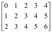
Reducing the spatial domain of an array while leaving the cell values unchanged is called trimming. Array dimension remains unchanged. Attempting to extend or intersect the array’s spatial domain will lead to an error; use the extend function in this case.
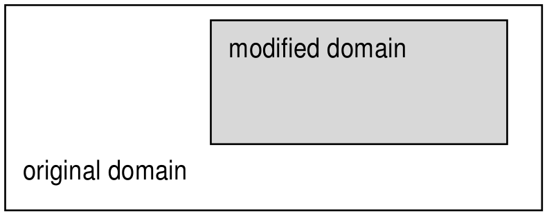
Figure 4.6 Spatial domain modification through trimming (2-D example)
Syntax
mddExp [ mintervalExp ]
Examples
The following query returns cutouts from the area [120: 160 , 55 : 75]
of all images in collection mr (see Figure 4.7).
select mr[ 120:160, 55:75 ]
from mr
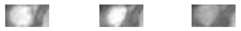
Figure 4.7 Trimming result
4.10.2.2. Section
A section allows to extract lower-dimensional layers (“slices”) from an array.
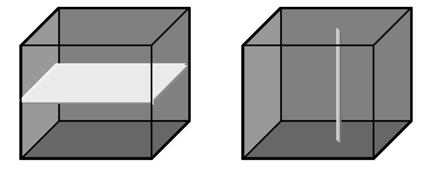
Figure 4.8 Single and double section through 3-D array, yielding 2-D and 1-D sections.
A section is accomplished through a trim expression by indicating the slicing position rather than a selection interval. A section can be made in any dimension within a trim expression. Each section reduces the dimension by one.
Like with trimming, a section must be within the spatial domain of the array, otherwise an error indicating that the subset domain extends outside of the array spatial domain will be thrown.
Syntax
mddExp [ integerExp_0 , ... , integerExp_n ]
This makes sections through mddExp at positions integerExp_i for each dimension i.
Example
The following query produces a 2-D section in the 2nd dimension of a 3-D cube:
select Images3D[ 0:256, 10, 0:256 ]
from Images3D
Note
If a section is done in every dimension of an array, the result is one single cell. This special case resembles array element access in programming languages, e.g., C/C++. However, in rasql the result still is an array, namely one with zero dimensions and exactly one element.
Example
The following query delivers a set of 0-D arrays containing single pixels, namely the ones with coordinate [100,150]:
select mr[ 100, 150 ]
from mr
4.10.2.3. Trim Wildcard Operator “*”
An asterisk “*” can be used as a shorthand for an sdom() invocation in a trim expression; the following phrases all are equivalent:
a [ *:*, *:* ] = a [ sdom(a)[0] , sdom(a)[1] ]
               = a [ sdom(a)[0].lo : sdom(a)[0].hi ,
                     sdom(a)[1].lo : sdom(a)[1].hi ]
An asterisk “*” can appear at any lower or upper bound position within a trim expression denoting the current spatial domain boundary. A trim expression can contain an arbitrary number of such wildcards. Note, however, that an asterisk cannot be used for specifying a section.
Example
The following are valid applications of the asterisk operator:
select mr[ 50:*, *:200 ]
from mr

select mr[ *:*, 10:150 ]
from mr
The next is illegal because it attempts to use an asterisk in a section:
select mr[ *, 100:200 ] -- illegal "*" usage in dimension 0
from mr
Note
It is well possible (and often recommended) to use an array’s spatial domain or part of it for query formulation; this makes the query more general and, hence, allows to establish query libraries. The following query cuts away the rightmost pixel line from the images:
select mr[ *:*, *:sdom(mr)[1].hi - 1 ]   -- good, portable
from mr
In the next example, conversely, trim bounds are written explicitly; this query’s trim expression, therefore, cannot be used with any other array type.
select mr[ 0:767, 0:1023 ]               -- bad, not portable
from mr
One might get the idea that the last query evaluates faster. This, however, is not the case; the server’s intelligent query engine makes the first version execute at just the same speed.
4.10.2.4. Positionally-independent Subsetting
Rasdaman supports positionally-independent subsetting like in WCPS and SQL/MDA, where for each trim/slice the axis name is indicated as well, e.g.
select mr2[d0(0:100), d1(50)] from mr2
The axis names give a reference to the addressed axes, so the order doesn’t matter anymore. This is equivalent:
select mr2[d1(50), d0(0:100)] from mr2
Furthermore, not all axes have to be specified. Any axes which are not specified default to “:”. For example:
select mr2[d1(50)] from mr2
=
select mr2[d0(*:*), d1(50)] from mr2
The two subset formats cannot be mixed, e.g. this is an error:
select mr2[d0(0:100), 50] from mr2
4.10.2.5. Shifting a Spatial Domain
Rasdaman provides built-in functions to transpose an array: its spatial domain remains unchanged in shape, but all cell contents simultaneously are moved to another location in n-dimensional space. Cell values themselves remain unchanged.
Syntax
shift( mddExp , pointExp )          (1a)
shift_by( mddExp , pointExp )       (1b)

shift_to( mddExp , pointExp )       (2)
The shift functions accept an mddExp and a pointExp and return an array whose spatial domain is shifted either
by the vector given by the pointExp in variants (1a) and (1b), or
to a new origin given by the pointExp in variant (2)
The dimension of pointExp must be equal to the dimension of the mddExp.
Examples
The following expression evaluates to an array with spatial domain
[3:13, 4:24] containing the same values as the original array a.
shift( a[ 0:10, 0:20 ], [ 3, 4 ] )

shift_by( a[ 0:10, 0:20 ], [ 3, 4 ] )
The following example shifts the array operand’s spatial domain
[ 5:15, 100:120 ] to a domain at origin [ 0, 0 ] (i.e.
[ 0:10, 0:20 ])
shift_to( a[ 5:15, 100:120 ], [ 0, 0 ] )
4.10.2.6. Extending a Spatial Domain
Function extend() enlarges a given MDD with the domain specified. The domain for extending must, for every boundary element, be at least as large as the MDD’s domain boundary. The new MDD contains 0 values in the extended part of its domain and the MDD’s original cell values within the MDD’s domain.
Syntax
extend( mddExp , mintervalExp )
The function accepts an mddExp and a mintervalExp and returns an array whose spatial domain is extended to the new domain specified by mintervalExp. The result MDD has the same cell type as the input MDD.
Precondition:
sdom( mddExp ) contained in mintervalExp
Example
Assuming that MDD a has a spatial domain of [0:50, 0:25], the following
expression evaluates to an array with spatial domain [-100:100, -50:50],
a‘s values in the subdomain [0:50, 0:25], and 0 values at the
remaining cell positions.
extend( a, [-100:100, -50:50] )
4.10.2.7. Geographic projection
4.10.2.7.1. Overview
“A map projection is any method of representing the surface of a sphere or other three-dimensional body on a plane. Map projections are necessary for creating maps. All map projections distort the surface in some fashion. Depending on the purpose of the map, some distortions are acceptable and others are not; therefore different map projections exist in order to preserve some properties of the sphere-like body at the expense of other properties.” (Wikipedia)
Each coordinate tieing a geographic object, map, or pixel to some position on earth (or some other celestial object, for that matter) is valid only in conjunction with the Coordinate Reference System (CRS) in which it is expressed. For 2-D Earth CRSs, a set of CRSs and their identifiers is normatively defined by the OGP Geomatics Committee, formed in 2005 by the absorption into OGP of the now-defunct European Petroleum Survey Group (EPSG). By way of tradition, however, this set of CRS definitions still is known as “EPSG”, and the CRS identifiers as “EPSG codes”. For example, EPSG:4326 references the well-known WGS84 CRS.
4.10.2.7.2. The project() function
Assume an MDD object M and two CRS identifiers C1 and C2 such as
“EPSG:4326”. The project() function establishes an output MDD, with same
dimension as M, whose contents is given by projecting M from CRS C1
into CRS C2.
The project() function comes in several variants based on the provided
input arguments
(1) project( mddExpr, boundsIn, crsIn, crsOut )

(2) project( mddExpr, boundsIn, crsIn, crsOut, resampleAlg )

(3) project( mddExpr, boundsIn, crsIn, boundsOut, crsOut,
                      widthOut, heightOut )

(4) project( mddExpr, boundsIn, crsIn, boundsOut, crsOut,
                      widthOut, heightOut, resampleAlg, errThreshold )

(5) project( mddExpr, boundsIn, crsIn, boundsOut, crsOut,
                      xres, yres)

(6) project( mddExpr, boundsIn, crsIn, boundsOut, crsOut,
                      xres, yres, resampleAlg, errThreshold )
where
mddExpr- MDD object to be reprojected.boundsIn- geographic bounding box given as a string of comma-separated floating-point values of the format:"xmin, ymin, xmax, ymax".crsIn- geographic CRS as a string. Internally, theproject()function is mapped to GDAL; hence, it accepts the same CRS formats as GDAL:Well Known Text (as per GDAL)
“EPSG:n”
“EPSGA:n”
“AUTO:proj_id,unit_id,lon0,lat0” indicating OGC WMS auto projections
“
urn:ogc:def:crs:EPSG::n” indicating OGC URNs (deprecated by OGC)PROJ.4 definitions
well known names, such as NAD27, NAD83, WGS84 or WGS72.
WKT in ESRI format, prefixed with “ESRI::”
“IGNF:xxx” and “+init=IGNF:xxx”, etc.
Since recently (v1.10), GDAL also supports OGC CRS URLs, OGC’s preferred way of identifying CRSs.
boundsOut- geographic bounding box of the projected output, given in the same format asboundsIn. This can be “smaller” than the input bounding box, in which case the input will be cropped.crsOut- geographic CRS of the result, in same format ascrsIn.widthOut,heightOut- integer grid extents of the result; the result will be accordingly scaled to fit in these extents.xres,yres- axis resolution in target georeferenced units.
resampleAlg- resampling algorithm to use, equivalent to the ones in GDAL:- near
Nearest neighbour (default, fastest algorithm, worst interpolation quality).
- bilinear
Bilinear resampling (2x2 kernel).
- cubic
Cubic convolution approximation (4x4 kernel).
- cubicspline
Cubic B-spline approximation (4x4 kernel).
- lanczos
Lanczos windowed sinc (6x6 kernel).
- average
Average of all non-NODATA contributing pixels. (GDAL >= 1.10.0)
- mode
Selects the value which appears most often of all the sampled points. (GDAL >= 1.10.0)
- max
Selects the maximum value from all non-NODATA contributing pixels. (GDAL >= 2.0.0)
- min
Selects the minimum value from all non-NODATA contributing pixels. (GDAL >= 2.0.0)
- med
Selects the median value of all non-NODATA contributing pixels. (GDAL >= 2.0.0)
- q1
Selects the first quartile value of all non-NODATA contributing pixels. (GDAL >= 2.0.0)
- q3
Selects the third quartile value of all non-NODATA contributing pixels. (GDAL >= 2.0.0)
errThreshold- error threshold for transformation approximation (in pixel units - defaults to 0.125).
Example
The following expression projects the MDD worldMap with bounding box
“-180, -90, 180, 90” in CRS EPSG 4326, into EPSG 54030:
project( worldMap, "-180, -90, 180, 90", "EPSG:4326", "EPSG:54030" )
The next example reprojects a subset of MDD Formosat with geographic
bbox “265725, 2544015, 341595, 2617695” in EPSG 32651, to bbox
“120.630936455 23.5842129067 120.77553782 23.721772322” in EPSG 4326 fit into
a 256 x 256 pixels area. The resampling algorithm is set to bicubic, and the
pixel error threshold is 0.1.
project( Formosat[ 0:2528, 0:2456 ],
  "265725, 2544015, 341595, 2617695", "EPSG:32651",
  "120.630936455 23.5842129067 120.77553782 23.721772322", "EPSG:4326",
  256, 256, cubic, 0.1 )
Limitations
Only 2-D arrays are supported. For multiband arrays, all bands must be of the same cell type.
4.10.2.7.3. Notes
Reprojection implies resampling of the cell values into a new grid, hence usually they will change.
As for the resampling process typically a larger area is required than the reprojected data area itself, it is advisable to project an area smaller than the total domain of the MDD.
Per se, rasdaman is a domain-agnostic Array DBMS and, hence, does not
know about CRSs; specific geo semantics is added by rasdaman’s petascope
layer. However, for the sake of performance, the
reprojection capability – which in geo service practice is immensely important
– is pushed down into rasdaman, rather than doing reprojection in
petascope’s Java code. To this end, the project() function provides rasdaman
with enough information to perform a reprojection, however, without
“knowing” anything in particular about geographic coordinates and CRSs.
One consequence is that there is no check whether this lat/long project is
applied to the proper axis of an array; it is up to the application (usually:
petascope) to handle axis semantics.
One consequence is that there is no check whether this lat/long project is applied to the proper axis of an array; it is up to the application (usually: petascope) to handle axis semantics.
4.10.3. Clipping Operations
Clipping is a general operation covering polygon clipping, linestring
selection, polytope clipping, curtain queries, and corridor queries. Presently,
all operations are available in rasdaman via the clip function.
4.10.3.1. Polygons
4.10.3.1.1. Syntax
select clip( c, polygon(( list of WKT points )) )
from coll as c
The input consists of an MDD expression and a list of WKT points, which determines the set of vertices of the polygon. Polygons are assumed to be closed with positive area, so the first vertex need not be repeated at the end, but there is no problem if it is. The algorithms used support polygons with self-intersection and vertex re-visitation.
Polygons may have interiors defined, such as
polygon( ( 0 0, 9 0, 9 9, 0 9, 0 0),
         ( 3 3, 7 3, 7 7, 3 7, 3 3 ) )
which would describe the annular region of the box [0:9,0:9] with the
interior box [3:7,3:7] removed. In this case, the interior polygons (there
may be many, as it forms a list) must not intersect the exterior polygon.
The clip bounding box must intersect the spatial domain of the MDD. The clipped areas that extend outside of the MDD will be set to null values.
4.10.3.2. Multipolygons
4.10.3.2.1. Syntax
select clip( c, multipolygon((( list of WKT points )),(( list of WKT points ))*) )
from coll as c
The input consists of an MDD expression and a list of polygons defined by list of WKT points. The assumptions about polygons are same as the ones for Polygon.
4.10.3.2.2. Return type
The output of a polygon query is a new array with dimensions corresponding to the bounding box of the polygon vertices. In case of Multipolygon, the new array have dimensions corresponding to closure of bounding boxes of every individual polygon, which domain intersects the collection’s spatial domain. The data in the array consists of null values where cells lie outside the polygon or MDD (or 0 values if no null values are associated with the array) and otherwise consists of the data in the collection where the corresponding cells lie inside the polygon. This could change the null values stored outside the polygon from one null value to another null value, in case a range of null values is used. By default, the first available null value will be utilized for the complement of the polygon.
An illustrative example of a polygon clipping is the right triangle with
vertices located at (0,0,0), (0,10,0) and (0,10,10), which can be
selected via the following query:
select clip( c, polygon((0 0 0, 0 10 0, 0 10 10)) )
from coll as c
4.10.3.2.3. Oblique polygons with subspacing
In case all the points in a polygon are coplanar, in some MDD object d of
higher dimension than 2, users can first perform a subspace operation on d
which selects the 2-D oblique subspace of d containing the polygon. For
example, if the polygon is the triangle polygon((0 0 0, 1 1 1, 0 1 1, 0 0 0)),
this triangle can be selected via the following query:
select clip( subspace(d, (0 0 0, 1 1 1, 0 1 1) ),
             polygon(( 0 0, 1 1 , 0 1 , 0 0)) )
from coll as d
where the result of subspace(d) is used as the domain of the polygon. For
more information look in Subspace Queries.
4.10.3.3. Linestrings
4.10.3.3.1. Syntax
select clip( c, linestring( list of WKT points ) ) [ with coordinates ]
from coll as c
The input parameter c refers to an MDD expression of dimension equal to the
dimension of the points in the list of WKT points. The list of WKT points
consists of parameters such as linestring(0 0, 19 -3, 19 -21), which would
describe the 3 endpoints of 2 line segments sharing an endpoint at 19 -3, in
this case.
4.10.3.3.2. Return type
The output consists of a 1-D MDD object consisting of the points selected along
the path drawn out by the linestring. The points are selected using a Bresenham
Line Drawing algorithm which passes through the spatial domain in the MDD
expression c, and selects values from the stored object. In case the
linestring spends some time outside the spatial domain of c, the first
null value will be used to fill the result of the linestring, just as in polygon
clipping.
When with coordinates is specified, in addition to the original cell values
the coordinate values are also added to the result MDD. The result cell type for
clipped MDD of dimension N will be composite of the following form:
If the original cell type
elemtypeis non-composite:{ long d1, ..., long dN, elemtype value }
Otherwise, if the original cell type is composite of
Mbands:{ long d1, ..., long dN, elemtype1 elemname1, ..., elemetypeM elemnameM }
4.10.3.3.3. Example
Select a Linestring from rgb data with coordinates. First two values of each
cell in the result are the x/y coordinates, with following values (three in this
case for RGB data) are the cell values of the clip operation to which
with coordinates is applied.
select encode(
    clip( c, linestring(0 19, 19 24, 12 17) ) with coordinates, "json")
from rgb as c
Result:
["0 19 119 208 248","1 19 119 208 248","2 20 119 208 248", ...]
The same query without specifying with coordinates:
select encode(
    clip( c, linestring(0 19, 19 24, 12 17) ), "json")
from rgb as c
results in
["119 208 248","119 208 248","119 208 248", ...]
4.10.3.4. Curtains
4.10.3.4.1. Syntax
select clip( c, curtain( projection(dimension pair),
                         polygon(( ... )) ) )
from coll as c
and
select clip( c, curtain( projection(dimension list),
                         linestring( ... ) ) )
from coll as c
The input in both variants consists of a dimension list corresponding to the
dimensions in which the geometric object, either the polygon or the linestring,
is defined. The geometry object is defined as per the above descriptions;
however, the following caveat applies: the spatial domain of the mdd expression
is projected along the projection dimensions in the projection(dimension
list). For a polygon clipping, which is 2-D, the dimension list is a pair of
values such as projection(0, 2) which would define a polygon in the axial
dimensions of 0 and 2 of the MDD expression c. For instance, if the spatial
domain of c is [0:99,0:199,0:255], then this would mean the domain upon
which the polygon is defined would be [0:99,0:255].
4.10.3.4.2. Return type
The output consists of a polygon clipping at every slice of the spatial domain
of c. For instance, if the projection dimensions of (0, 2) are used for
the same spatial domain of c above, then a polygon clipping is performed at
every slice of c of the form [0:99,x,0:255] and appended to the result
MDD object, where there is a slice for each value of x in [0:199].
4.10.3.5. Corridors
4.10.3.5.1. Syntax
select clip( c, corridor( projection(dimension pair),
                          linestring( ... ),
                          polygon(( ... )) ) )
from coll as c
and
select clip( c, corridor( projection(dimension pair),
                          linestring( ... ),
                          polygon(( ... )),
                          discrete ) )
from coll as c
The input consists of a dimension list corresponding to the dimensions in which the geometric object, in this case a polygon, is defined. The linestring specifies the path along which this geometric object is integrated. One slice is sampled at every point, and at least the first point of the linestring should be contained within the polygon to ensure a meaningful result (an error is thrown in case it is not). There is an optional discrete flag which modifies the output by skipping the extrapolation of the linestring data to interior points.
4.10.3.5.2. Return type
The output consists of a polygon clipping at every slice of the spatial domain
of c translated along the points in the linestring, where the first axis of
the result is indexed by the linestring points and the latter axes are indexed
by the mask dimensions (in this case, the convex hull of the polygon). The
projection dimensions are otherwise handled as in curtains; it is the spatial
offsets given by the linestring coordinates which impact the changes in the
result. In the case where the discrete parameter was utilized, the output is
indexed by the number of points in the linestring description in the query and
not by the extrapolated linestring, which uses a Bresenham algorithm to find
the grid points in between.
4.10.3.6. Subspace Queries
Here we cover the details of subspace queries in rasdaman. Much like slicing via a query such as
select c[0:9,1,0:9] from collection as c
the subspace query parameter allows users to extract a lower-dimensional dataset from an existing collection. It is capable of everything that a slicing query is capable of, and more. The limitation of slicing is that the selected data must lie either parallel or perpendicular to existing axes; however, with subspacing, users can arbitrarily rotate the axes of interest to select data in an oblique fashion. This control is exercised by defining an affine subspace from a list of vertices lying in the datacube. Rasdaman takes these points and finds the unique lowest-dimensional affine subspace containing them, and outputs the data closest to this slice, contained in the bounding box of the given points, into the resulting array.
Structure of the query:
select clip( c, subspace(list of WKT points) )
from coll as c
We can illustrate the usage with an example of two queries which are identical in output:
select clip( c, subspace(0 0 0, 1 0 0, 0 0 1) ) from coll as c

select c[0:1,0,0:1] from coll as c
This example will result in 1D array of sdom [0:99]:
select clip( c, subspace(19 0, 0 99) ) from test_rgb as c
This example will result in a a 2D array of sdom [0:7,0:19]:
select clip( c, subspace(0 0 0, 0 19 0, 7 0 7) )
from test_grey3d as c
and it will consist of the best integer lattice points reachable by the vectors
(1,0,1) and (0,1,0) within the bounding box domain of [0:7,0:19,0:7]
in test_grey3d.
Generally speaking, rasdaman uses the 1st point as a basepoint for an affine
subspace containing all given points, constructs a system of equations to
determine whether or not a point is in that subspace or not, and then searches
the bounding box of the given points for solutions to the projection operator
which maps [0:7,0:19,0:7] to [0:7,0:19]. The result dimensions are
chosen such that each search yields a unique real solution, and then rasdaman
rounds to the nearest integer cell before adding the value stored in that cell
to the result object.
Some mathematical edge cases:
Because of arithmetic on affine subspaces, the following two queries are fundamentally identical to rasdaman:
select clip( c, subspace(0 0 0, 1 1 0, 0 1 0) )
from test_grey3d as c

select clip( c, subspace(0 0 0, 1 0 0, 0 1 0) )
from test_grey3d as c
Rasdaman’s convention is to use the first point as the translation point, and constructs the vectors generating the subspace from the differences. There is no particular reason not to use another point in the WKT list; however, knowing this, users should be aware that affine subspaces differ slightly from vector subspaces in that the following two queries differ:
select clip( c, subspace(10 10 10, 0 0 10, 10 0 10) )
from test_grey3d as c

select clip( c, subspace(0 0 0, 10 10 0, 0 10 0) )
from test_grey3d as c
The two queries have the same result domains of [0:10,0:10], and the projection
for both lie on the first 2 coordinate axes since the 3rd coordinate remains
constant; however, the data selections differ because the subspaces generated by
these differ, even though the generating vectors of (1 1 0) and (0 1 0)
are the same.
Even though the bounding box where one searches for solutions is the same
between these two queries, there is no way to reach the origin with the vectors
(1 1 0) and (0 1 0) starting at the base point of (10 10 10) because
neither vector can impact the 3rd coordinate value of 10; similarly, starting at
(0 0 0) must leave the third coordinate fixed at 0. There is nothing special
about choosing the first coordinate as our base point – the numbers might
change, but the resulting data selections in both queries would remain constant.
The following two queries generate the same subspace, but the latter has a larger output domain:
select clip( c, subspace(0 0 0, 1 1 0, 0 1 0) )
from test_grey3d as c

select clip( c, subspace(0 0 0, 1 1 0, 0 1 0, 0 0 0, 1 2 0) )
from test_grey3d as c
As much redundancy as possible is annihilated during a preprocessing stage which uses a Gram-Schmidt procedure to excise extraneous data imported during query time, and with this algorithm, rasdaman is able to determine the correct dimension of the output domain.
Some algorithmic caveats:
The complexity of searching for a solution for each result cell is related to
the codimension of the affine subspace, and not the dimension of the affine
subspace itself. In fact, if k is the difference between the dimension of the
collection array and the dimension of the result array, then each cell is
determined in O(k^2) time. Preprocessing happens once for the entire query,
and occurs in O(k^3) time. There is one exception to the codimensionality
considerations: a 1-D affine subspace (also known as a line segment) is selected
using a multidimensional generalization of the Bresenham Line Algorithm, and so
the results are determined in O(n) time, where n is the dimension of the
collection.
Tip: If you want a slice which is parallel to axes, then you are better off using the classic slicing style of:
select c[0:19,0:7,0] from collection as c
as the memory offset computations are performed much more efficiently.
4.10.4. Induced Operations
Induced operations allow to simultaneously apply a function originally working on a single cell value to all cells of an MDD. The result MDD has the same spatial domain, but can change its base type.
Examples
img.green + 5 c
This expression selects component named “green” from an RGB image and adds 5 (of type char, i.e., 8 bit) to every pixel.
img1 + img2
This performs pixelwise addition of two images (which must be of equal spatial domain).
Induction and structs
Whenever induced operations are applied to a composite cell structure (“structs” in C/C++), then the induced operation is executed on every structure component. If some cell structure component turns out to be of an incompatible type, then the operation as a whole aborts with an error.
For example, a constant can be added simultaneously to all components of an RGB image:
select rgb + 5
from rgb
Induction and complex
Complex numbers, which actually form a composite type supported as a base type, can be accessed with the record component names re and im for the real and the imaginary part, resp.
Example
The first expression below extracts the real component, the second one the imaginary part from a complex number c:
c.re
c.im
4.10.4.1. Unary Induction
Unary induction means that only one array operand is involved in the expression. Two situations can occur: Either the operation is unary by nature (such as boolean not); then, this operation is applied to each array cell. Or the induce operation combines a single value (scalar) with the array; then, the contents of each cell is combined with the scalar value.
A special case, syntactically, is the struct/complex component selection (see next subsection).
In any case, sequence of iteration through the array for cell inspection is chosen by the database server (which heavily uses reordering for query optimisation) and not known to the user.
Syntax
unaryOp mddExp
mddExp binaryOp scalarExp
scalarExp binaryOp mddExp
Example
The red images of collection rgb with all pixel values multiplied by 2:
select rgb.red * 2c
from rgb
Note that the constant is marked as being of type char so that the result type
is minimized (short). Omitting the “c” would lead to an addition of long
integer and char, resulting in long integer with 32 bit per pixel. Although
pixel values obviously are the same in both cases, the second alternative
requires twice the memory space. For more details visit the
Type Coercion Rules section.
4.10.4.2. Struct Component Selection
Component selection from a composite value is done with the dot operator well-known from programming languages. The argument can either be a number (starting with 0) or the struct element name. Both statements of the following example would select the green plane of the sample RGB image.
This is a special case of a unary induced operator.
Syntax
mddExp.attrName
mddExp.intExp
Examples
select rgb.green
from rgb

select rgb.1
from rgb

Figure 4.9 RGB image and green component
Note
Aside of operations involving base types such as integer and boolean, combination of complex base types (structs) with scalar values are supported. In this case, the operation is applied to each element of the structure in turn.
Examples
The following expression reduces contrast of a color image in its red, green, and blue channel simultaneously:
select rgb / 2c
from rgb
An advanced example is to use image properties for masking areas in this image. In the query below, this is done by searching pixels which are “sufficiently green” by imposing a lower bound on the green intensity and upper bounds on the red and blue intensity. The resulting boolean matrix is multiplied with the original image (i.e., componentwise with the red, green, and blue pixel component); the final image, then, shows the original pixel value where green prevails and is {0,0,0} (i.e., black) otherwise (Figure 4.10)
select rgb * ( (rgb.green > 130c) and
               (rgb.red   < 110c) and
               (rgb.blue  < 140c) )
from rgb

Figure 4.10 Suppressing “non-green” areas
Note
This mixing of boolean and integer is possible because the usual C/C++ interpretation of true as 1 and false as 0 is supported by rasql.
4.10.4.3. Binary Induction
Binary induction means that two arrays are combined.
Syntax
mddExp binaryOp mddExp
Example
The difference between the images in the mr collection and the image in
the mr2 collection:
select mr - mr2
from mr, mr2
Note
Two cases have to be distinguished:
Both left hand array expression and right hand array expression operate on the same array, for example:
select rgb.red - rgb.green
from rgb
In this case, the expression is evaluated by combining, for each coordinate position, the respective cell values from the left hand and right hand side.
Left hand array expression and right hand array expression operate on different arrays, for example:
select mr - mr2
from mr, mr2
This situation specifies a cross product between the two collections involved. During evaluation, each array from the first collection is combined with each member of the second collection. Every such pair of arrays then is processed as described above.
Obviously the second case can become computationally very expensive, depending on the size of the collections involved - if the two collections contain n and m members, resp., then n*m combinations have to be evaluated.
4.10.4.4. Case statement
The rasdaman case statement serves to model n-fold case distinctions based on the SQL92 CASE statement which essentially represents a list of IF-THEN statements evaluated sequentially until either a condition fires and delivers the corresponding result or the (mandatory) ELSE alternative is returned.
In the simplest form, the case statement looks at a variable and compares it to different alternatives for finding out what to deliver. The more involved version allows general predicates in the condition.
This functionality is implemented in rasdaman on both scalars (where it resembles SQL) and on MDD objects (where it establishes an induced operation). Due to the construction of the rasql syntax, the distinction between scalar and induced operations is not reflected explicitly in the syntax, making query writing simpler.
Syntax
Variable-based variant:
case generalExp
when scalarExp then generalExp
[ when scalarExp then generalExp ]*
else generalExp
end
All generalExps must be of a compatible type.
Expression-based variant:
case
when booleanExp then generalExp
[ when scalarExp then generalExp ]*
else generalExp
end
All generalExp’s must evaluate to a compatible type.
Example
Traffic light classification of an array object can be done as follows.
select
  case
  when mr > 150 then { 255c, 0c, 0c }
  when mr > 100 then { 0c, 255c, 0c }
  else               { 0c, 0c, 255c }
  end
from mr
This is equivalent to the following query; note that this query is less efficient due to the increased number of operations to be evaluated, the expensive multiplications, etc:
select
  (mr > 150)                { 255c, 0c, 0c }
+ (mr <= 150 and mr > 100)  { 0c, 255c, 0c }
+ (mr <= 100)               { 0c, 0c, 255c }
from mr
Restrictions
In the current version, all MDD objects participating in a case statement must have the same tiling. Note that this limitation can often be overcome by factoring divergingly tiled arrays out of a query, or by resorting to the query equivalent in the above example using multiplication and addition.
4.10.4.5. Induction: All Operations
Below is a complete listing of all cell level operations that can be induced, both unary and binary. Supported operand types and rules for deriving the result types for each operation are specified in Type Coercion Rules.
- +, -, *, /
For each cell within some MDD value (or evaluated MDD expression), add it with the corresponding cell of the second MDD parameter. For example, this code adds two (equally sized) images:
img1 + img2
- div, mod
In contrast to the previous operators, div and mod are binary functions. The difference of
divto/is that in the case of integer inputs,divresults in integer result, and hence must check for division with 0, in which case an error would be thrown. The behaviour ofmodis the same. Example usage:div(a, b) mod(a, b)
- pow, power
The power function can be written as
poworpower. The signature is:pow( base, exp )
where base and is an MDD or scalar, and exp is an MDD or scalar of non-composite type.
- =, <, >, <=, >=, !=
For two MDD values (or evaluated MDD expressions), compare for each coordinate the corresponding cells to obtain the Boolean result indicated by the operation.
These comparison operators work on all atomic cell types.
On composite cells, only
=and!=are supported; both operands must have a compatible cell structure. In this case, the comparison result is the conjunction (“and” connection) of the pairwise comparison of all cell components.- and, or, xor, is, not
For each cell within some Boolean MDD (or evaluated MDD expression), combine it with the second MDD argument using the logical operation
and,or, orxor. Theisoperation is equivalent to=(see below). The signature of the binary induced operation isis, and, or, xor: mddExp, intExp -> mddExp
Unary function
notnegates each cell value in the MDD.- min, max
For two MDD values (or evaluated MDD expressions), take the minimum / maximum for each pair of corresponding cell values in the MDDs.
Example:
a min b
For struct valued MDD values, struct components in the MDD operands must be pairwise compatible; comparison is done in lexicographic order with the first struct component being most significant and the last component being least significant.
- overlay
The overlay operator allows to combine two equally sized MDDs by placing the second one “on top” of the first one, informally speaking. Formally, overlaying is done in the following way:
wherever the second operand’s cell value is not zero and not null, the result value will be this value.
wherever the second operand’s cell value is zero or null, the first argument’s cell value will be taken.
This way stacking of layers can be accomplished, e.g., in geographic applications. Consider the following example:
ortho overlay tk.water overlay tk.streets
When displayed the resulting image will have streets on top, followed by water, and at the bottom there is the ortho photo.
Strictly speaking, the overlay operator is not atomic. Expression
a overlay b
is equivalent to
(b is not null) * b + (b is null) * a
However, on the server the overlay operator is executed more efficiently than the above expression.
- bit(mdd, pos)
For each cell within MDD value (or evaluated MDD expression) mdd, take the bit with nonnegative position number pos and put it as a Boolean value into a byte. Position counting starts with 0 and runs from least to most significant bit. The bit operation signature is
bit: mddExp, intExp -> mddExp
In C/C++ style,
bit(mdd, pos)is equivalent tomdd >> pos & 1.
- Arithmetic, trigonometric, and exponential functions
The following advanced arithmetic functions are available with the obvious meaning, each of them accepting an MDD object (except
arctan2which expects two floating-point operands of the same type):abs() sqrt() exp() log() ln() sin() cos() tan() sinh() cosh() tanh() arcsin() arccos() arctan() arctan2() ceil() floor() round()
Exceptions
Generally, on domain error or other invalid cell values these functions will not throw an error, but result in NaN or similar according to IEEE floating-point arithmetic. Internally the rasdaman implementation calls the corresponding C++ functions, so the C++ documentation applies.
The
ceil,floor, androundfunctions are applicable only on floating-point arguments and have no effect on other atomic types (e.g. char). On multi-band arguments with bands of mixed floating-point and other base types, these function are not applicable and throw an error.- cast
Sometimes the desired ultimate scalar type or MDD cell type is different from what the MDD expression would suggest. To this end, the result type can be enforced explicitly through the cast operator.
The syntax is:
(newType) generalExp
where newType is the desired result type of expression generalExp.
Like in programming languages, the cast operator converts the result to the desired type if this is possible at all. For example, the following scalar expression, without cast, would return a double precision float value; the cast makes it a single precision value:
(float) avg_cells( mr )
Both scalar values and MDD can be cast; in the latter case, the cast operator is applied to each cell of the MDD yielding an array over the indicated type.
The cast operator also works properly on composite cell structures. In such a case, the cast type is applied to every component of the cell. For example, the following expression converts the pixel type of an (3x8 bit) RGB image to an image where each cell is a structure with three long components:
(long) rgb
Obviously in the result structure all components will bear the same type. In addition, the target type can be a user-defined composite type, e.g. the following will cast the operand to {1c, 2c, 3c}:
(RGBPixel) {1c, 2l, 3.0}
Casting from larger to smaller integer type
If the new type is smaller than the value’s type, i.e. not all values can be represented by it, then standard C++ casting will typically lead to strange results due to wrap around for unsigned and implementation-defined behavior for a signed types. For example, casting int 1234 to char in C++ will result in 210, while the possible range would be 0 - 255.
Rasdaman implements a more reasonable cast behavior in this case: if the value is larger than the maximum value representable by the new type, then the result is the maximum value (e.g. 255 in the previous example); analogously, if the value is smaller than the minimum possible value, then the result is the minimum value.
This is implemented only on integer types and entails a small performance penalty in comparison to raw C++ as up to two comparisons per cell (with the maximum and minimum) are necessary when casting.
Restrictions
On base type complex, only the following operations are available right now:
+ - * /
4.10.5. Scaling
Shorthand functions are available to scale multidimensional objects. They receive an array as parameter, plus a scale indicator. In the most common case, the scaling factor is an integer or float number. This factor then is applied to all dimensions homogeneously. For a scaling with individual factors for each dimension, a scaling vector can be supplied which, for each dimension, contains the resp. scale factor. Alternatively, a target domain can be specified to which the object gets scaled.
Syntax
scale( mddExp, intExp )
scale( mddExp, floatExp )
scale( mddExp, intVector )
scale( mddExp, mintervalExp )
Examples
The following example returns all images of collection mr where each
image has been scaled down by a factor of 2.
select scale( mr, 0.5 )
from mr
Next, mr images are enlarged by 4 in the first dimension and 3 in the second dimension:
select scale( mr, [ 4, 3 ] )
from mr
In the final example, mr images are scaled to obtain 100x100 thumbnails (note that this can break aspect ratio):
select scale( mr, [ 0:99, 0:99 ] )
from mr
Note
Function scale() breaks tile streaming, it needs to load all tiles
affected into server main memory. In other words, the source argument of
the function must fit into server main memory. Consequently, it is not
advisable to use this function on very large items.
Note
Currently only nearest neighbour interpolation is supported for scaling. It uses floor for rounding to integer coordinates when finding the nearest neighbour. So it has same behavior as OpenCV, for example, as explained in this blog post.
4.10.6. Concatenation
Concatenation of two arrays “glues” together arrays by lining them up along an axis.
This can be achieved with a shorthand function, concat, which for
convenience is implemented as an n-ary operator accepting an unlimited number
of arrays of the same base type. The operator takes the input arrays, lines
them up along the concatenation dimension specified in the request, and outputs
one result array. To this end, each input array from the second one on is
shifted to the origin of the first one, except along the concatenation
dimension where it’s shifted so that the lower bound of the current array is
right after the upper bound of the previous array.
The resulting array’s dimensionality is equal to the input array dimensionality.
The resulting array extent is the sum of all extents along the concatenation dimension, and the extent of the input arrays in all other dimensions; the origin is same as the origin of the first input array.
The resulting array cell type is same as the cell types of the input arrays.
Constraints
All participating arrays must have the same number of dimensions.
All participating arrays must have identical extents in all dimensions, except the dimension along which concatenation is performed.
Input arrays must have the same cell types, i.e. concatenating a char and float arrays is not possible and requires explicit casting to a common type.
Syntax
concat mddExp
with mddExp
[ with mddExp ]*
along integer
Examples
The following query returns the concatenation of all images of collection mr with themselves along the first dimension (Figure 4.11).
select concat mr with mr along 0
from mr
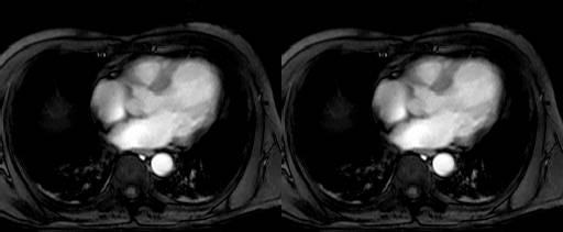
Figure 4.11 Query result of single concatenation
The next example returns a 2x2 arrangement of images (Figure 4.12):
select concat (concat mr with mr along 0)
with (concat mr with mr along 0)
along 1
from mr
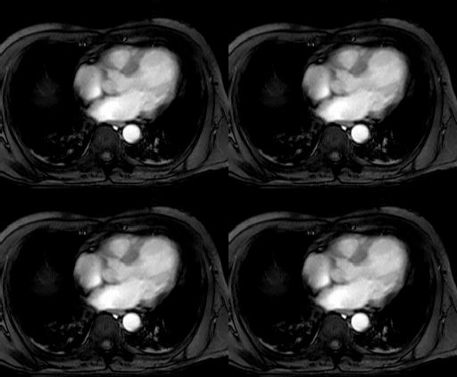
Figure 4.12 Query result of multiple concatenation
4.10.7. Transpose [RE]
The transpose operation is a fundamental matrix transformation that reorients data by flipping a matrix over its main diagonal, converting its rows into columns and vice versa. The transpose of an \(m \times n\) matrix \(A\), usually denoted \(A^T\), switches the row and column indices of elements producing an \(n \times m\) matrix. This simple re-indexing is crucial in linear algebra, as it underpins definitions of symmetry, dot products, and systems of linear equations.
The concept of transposition extends naturally to multidimensional arrays, where it generalizes to a permutation of axes. Instead of a single flip across a diagonal, transposing a higher-dimensional array involves swapping specified dimensions according to a newly defined order, thereby rearranging the data’s orientation in memory. This operation is essential in fields like machine learning and scientific computing.
Syntax
transpose(mddExp)               (1)
transpose(mddExp, pointExp)     (2)
The first operand is an expression resulting in a multidimensional array to be
transposed. If the second operand is specified, it is the new axis order as a
list of \(D\) axis indices, where \(D\) is the dimensionality of
mddExp. The axis indices are 0-based, i.e. the first axis of mddExp is
0, the second is 1, and so on.
Semantics
In both cases, mddExp can be an array of any dimension. Transposing 1-D
arrays is allowed but has no effect on the operand, i.e. the result is same as
the input array.
Alternative (1) is a shorthand for (2) with a pointExp of the form
\([D-1, D-2, \ldots, 0]\). In short, it reverses the axes of the array
operand.
Each axis of mddExp must be referenced exactly once in the list of axis
indices in pointExp. If an axis is not referenced, or is listed multiple
times, or an index is outside the \(0 \ldots D-1\) range, then an error is
returned.
The result is an array with a spatial domain determined by the new axis order as
given by pointExp. The total number of elements or their values does not
change from mddExp, only their positions. The cell type remains unchanged.
Performance
Due to how arrays are linearized in memory internally, transposing the last two axes of an array can be done efficiently and is therefore implemented with specialized routines that are heavily optimized to make use of CPU caches and SIMD capabilities (SSE/AVX on x86 platforms). So transposing 2-D arrays or the last two axes of n-D arrays is fast.
Transposing other axes on the other hand is done with generic code that is relatively expensive/slower.
In all cases tile streaming is preserved, i.e. a transpose operation is not blocking and is performed on multiple tiles in parallel.
Examples
The following query transposes the mr2 image:
select encode(transpose(mr2), "PNG")
from mr2
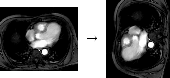
Figure 4.13 Transposing an image in the mr2 collection.
The exact same result is achieved with explicitly specifying the new axis order:
select encode(transpose(mr2, [1, 0]), "PNG")
from mr2
Swapping the last two axes of a 4-D array can be done with:
select transpose(c, [0, 1, 3, 2])
from test_4D as c
Or reversing the first three axes:
select transpose(c, [2, 1, 0, 3])
from test_4D as c
4.10.8. Quantiles [RE]
The rasql enterprise function quantile() delivers the q-quantile
distribution over a given array object.
Quantiles (cf. Wikipedia) are “points taken at regular intervals from the cumulative distribution function (CDF) of a random variable. Dividing ordered data into q essentially equal- sized data subsets is the motivation for q-quantiles; the quantiles are the data values marking the boundaries between consecutive subsets. Put another way, the k-th q-quantile for a random variable is the value x such that the probability that the random variable will be less than x is at most k/q and the probability that the random variable will be more than x is at most (q - k) / q = 1 - (k / q). There are q-1 of the q-quantiles, one for each integer k satisfying 0 < k < q.”
The quantile() function signature is
quantile: mddExpr, intExpr -> mddExpr
Given an MDD object M and a parameter Q, the quantile function sorts the data in increasing order, partitions the data in Q equal parts, and returns a 1-dimensional MDD object of size Q-1 and same type as the input object, which contains the boundary values between the consecutive parts.
Example
Assume an n-D MDD, M, of which we want to have all 100-quantiles (percentiles); this is written as
quantile(M, 100)
This expression results in a 1-D object containing 99 values, where the first value corresponds to the 1st percentile:
quantile(M, 100)[0]
and the 50th value to the 50th percentile:
quantile(M, 100)[49]
Since the 50th percentile is equivalent to the median (2-quantile), the above query is equivalent to
quantile(M, 2)[0]
Quantile fields
The quantile function can be used to derive quantile fields. For example, assume an x/y/t time series object T where x, y, and t have dimensions 0, 1, and 2, resp. The following expression obtains an x/y map of 95% percentiles (q=100) over time for each x/y location, thereby detecting anomalies over time:
marray x in sdom(T)[0], y in sdom(T)[1]
values quantile( T[ x, y ], 100)[94]
Limitations
Only arrays with an atomic cell type are supported currently.
Sorting of data is done in main memory so the size of a single quantile result array is limited to the server’s main memory.
4.10.9. Mosaicing arrays [RE]
The mosaic function merges multiple non-overlapping MDDs into a single
result MDD. Parts in the resulting spatial domain that do not intersect with
the spatial domain of any of the operand MDDs are set to NULL.
Syntax
mosaic(mdd_1, mdd_2, ..., mdd_n)
Preconditions
basetype(mdd\(_i\)) = basetype(mdd\(_j\)), for \(1 <= i,j <= n\)
dimension(mdd\(_i\)) = dimension(mdd\(_j\))
disjoint(sdom(mdd\(_i\)), sdom(mdd\(_j\))
compatible nullsets
Postconditions
basetype(result) = basetype(mdd\(_1\))
sdom(result) = union(sdom(mdd\(_i\)))
nullset(result) = nullset_union(mdd\(_i\))
Semantics
The mosaic function is equivalent to the following rasql expression:
MARRAY i in sdom(result)
VALUES CASE
         WHEN i IN sdom(mdd_1) THEN mdd_1[i]
         WHEN i IN sdom(mdd_2) THEN mdd_2[i]
         ...
         WHEN i IN sdom(mdd_n) THEN mdd_n[i]
         ELSE null
       END
Example
The 1s and 2s are two input MDDs, the ns in the result indicate NULLs.
  │                               │
  │   mdd_1       mdd_2           │   result
  │ ┌────────┐  ┌───────┐         │ ┌───────────────────┐
  │ │11111111│  │2222222│         │ │11111111nnnn2222222│
  │ │11111111│  │2222222│         │ │11111111nnnn2222222│
  │ │11111111│  └───────┘  ────►  │ │11111111nnnnnnnnnnn│
  │ │11111111│                    │ │11111111nnnnnnnnnnn│
  │ │11111111│                    │ │11111111nnnnnnnnnnn│
  │ └────────┘                    │ └───────────────────┘
  │                               │
  └───────────────────────────    └───────────────────────────
origin                          origin
4.10.10. SORT operator
The SORT operator allows to sort the slices along a given axis of an array.
This is done by calculating a rank value for each of the slices according to a
given ranking function, and then reordering the slices according to their
ranks in ascending (by default) or descending order.
Syntax
SORT generalExp
ALONG sortAxis AS sortAxisIterator [listingOrder]
BY cellExp
Where
sortAxis: integerLit | identifier
sortAxisIterator: identifier
listingOrder: ASC | DESC
The generalExp denotes the array to be sorted; arrays of any dimensionality
and type can be specified, or expressions that produce an array.
The sortAxis along which the array is sliced and reordered is specified in
the ALONG clause. It can be specified by axis name according to the MDD
type definition (e.g. x, y, Lat, …), or by an integer indicating its 0-based
order (0 for the first axis, 1 for the second, and so on). Additionally a
sortAxisIterator must be specified as an alias for addressing the axis in
the ranking function, e.g. in subsetting the generalExp into slices and
aggregating each into a rank. Depending on the optional listingOrder the
slices are sorted in ascending ASC (default if not specified) or descending
DESC order.
The cellExp in the BY clause is the slice ranking function. It must
result in an atomic scalar value for each point in the sort axis extent. Slices
for which the same rank is calculated retain their relative order as in the
input array (stable sorting). The sortAxisIterator can be used to reference
the points along the sortAxis.
The mechanics of the SORT expressions is perhaps more clearly explained via an
equivalence to an MARRAY constructor expression, which creates a 1D array of
ranks calculated by the cellExp for each point in the 1D domain created by
the extend of the sortAxis; then SORT sorts these ranks and the slices to
which they correspond in ascending or descending order. For example, if A is
a 3D array and we have the a SORT expression that reorders the slices along the
first axis by their average values:
SORT A
ALONG 0 AS sortAxis
BY avg_cells( A[ sortAxis[0], *:*, *:* ] )
then before the sorting is applied, first the ranks for each slice are calculated with an MARRAY:
MARRAY sortAxis in [ sdom(A)[0].lo : sdom(A)[0].hi ]
VALUES avg_cells( A[ sortAxis[0], *:*, *:* ] )
The sorting causes no change in the spatial domain, base type, or dimensionality in the result.
Examples
The following examples illustrate the syntax of the SORT operator;
raster2D and raster3D are 2D and 3D MDDs with axes x/y and t/x/y
respectively.
The following examples show the semantics of the sort operator. Array cells which contribute to the rank result are highlighted in red.
expand example
The following example shows how a 10x3 array of double floating-point values is sorted along its second axis in an ascending order by the minimum of all values in each slice.
SORT raster2D ALONG 1 AS i
BY min_cells(raster2D[*:*, i[0]])
The array looks as follows before and after sorting:
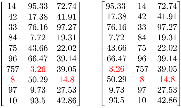
Figure 4.14 Minimum values in columns 0,1,2 are 8, 3.26, and 14.8 respectively, highlighted in red.
We observe that the sorting was a reordering of the slices along the second axis, represented by the columns.
expand example
By subsetting along an axis other than the sortAxis, we can further restrict
areas in the slices which contribute to the ranking function. For example, the
following 2 queries consider only the value at index positions 0 or 1,
respectively, along axis 1.
SORT raster2D ALONG 0 AS i
BY (raster2D2[i[0], 0])

SORT raster2D ALONG 0 AS i
BY (raster2D2[i[0], 1])
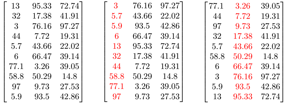
Figure 4.15 Sorting an array with further subsetting each slice along the sort axis.
expand example
You might also want to compare two values in a specific axis at once, at each slice, and sort by the minimum value between those, using an aggregate operation:
SORT raster2D ALONG 0 AS i
BY min_cells(raster2D2[i[0], 1:2])
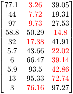
Figure 4.16 Sorting an array by the minimum value with further subsetting at a specific axis.
expand example
The next example, shows how a 3D array of double floating-point values for temperature is sorted along its first axis of time in a descending order, by the maximum temperature value in each latitude/longitude combination:
SORT weather ALONG 0 AS i DESC
BY max_cells(weather[i[0], *:*, *:*])
The datasheet looks as follows:
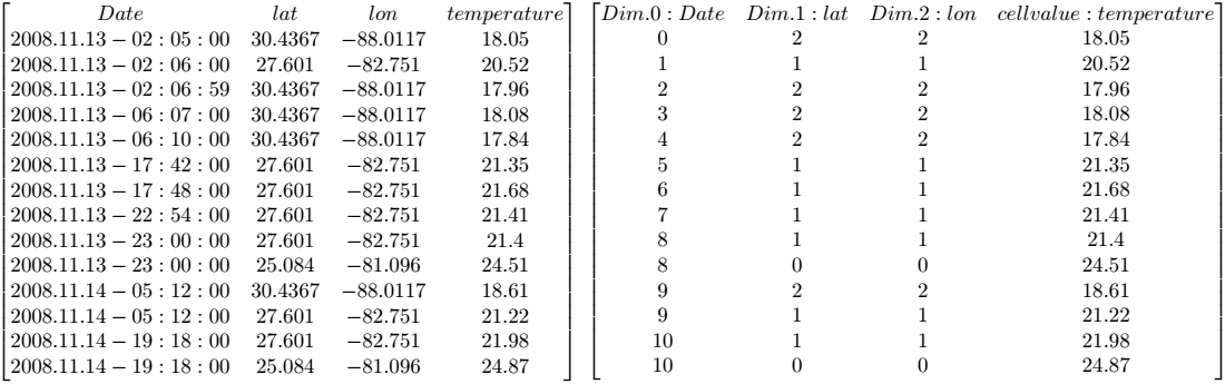
The first datasheet represents all the data that we have. The second offers a datacube interpretation of the available data. The first dimension is time, the second the latitude, and the third represents the longitude. In this example, the lat/lon are limited to 3 entries each. And the temperature is recorded at 11 unique timestamps. Thus, the data is represented using the available combinations of longitude and latitude (25.084,-81.096),(27.601,-82.751) and (30.4367,-88.0117), by (0,0), (1,1) and (2,2) respectively, each in their timestamp. All the cell values are recorded temperatures.
The following illustration represents a 3D array holding this data:
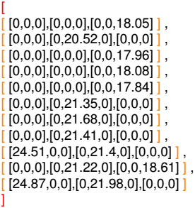
On the first timestamp, for instance, we have a temperature measurement of 18.05 degrees, for lat/lon (2,2), which represents (30.4367,-88.0117) of the original table. In the last timestamp, we have two temperature records, at (0,0) and at (1,1). If we had more measurements, they would fill in the zero-values.
After sorting, the array looks as follows:
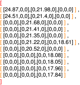
We observe that the time-slices have been sorted by their maximum value, in a descending manner.
One can also sort by a specific longitude/latitude combination, e.g:
SORT weather ALONG 0 AS i
BY weather[i[0], 0, 0] DESC
4.10.11. FLIP operator
The FLIP operator allows to reverse the values/slices of an MDD along a
particular axis. Similar to SORT, the array is sliced at the chosen axis.
The slices are then reordered in opposite order, resulting in an array
with no change in the spatial domain, base type, or dimensionality.
Syntax
FLIP generalExp ALONG flipAxis
Where
flipAxis: integerLit | identifier
The generalExp denotes the array argument; arrays of any dimensionality
and type can be specified (or expressions that produce an array).
The flipAxis along which the array is sliced and reordered in reverse order
is specified in the ALONG clause. It can be specified by axis name
according to the MDD type definition (e.g. x, y, Lat, …), or by an integer
indicating its 0-based order (0 for the first axis, 1 for the second, and so
on).
Examples
The following examples illustrate the syntax of the FLIP operator;
raster2D and raster3D are 2D and 3D MDDs with axes x/y and time/x/y
respectively.
The next example illustrates the inversion of the following array:
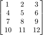
Flipping the array on its first axis with
FLIP raster2D ALONG 0
and flipping on the second axis with
FLIP raster2D ALONG 1
yields the following results, respectively:
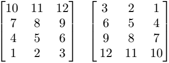
In a more visual example, applying the FLIP operation on the sample MRT imagery
collection mr2 will mirror the image vertically or horizontally. The
original image looks as follows:
flipping on the first axis with
FLIP mr2 ALONG 0
results in
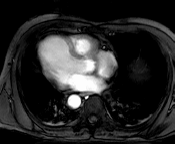
Figure 4.17 the image is mirrored on the vertical axis
and flipping on the second axis with
FLIP mr2 ALONG 1
results in
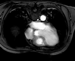
Figure 4.18 the image is mirrored on the horizontal axis
4.10.12. Condensers
Frequently summary information of some kind is required about some array, such as sum or average of cell values. To accomplish this, rasql provides the concept of condensers.
A condense operation (or short: condenser) takes an array and summarizes its values using a summarization function, either to a scalar value (e.g. computing the sum of all its cells), or to another array (e.g. summarizing a 3-D cube into a 2-D image by adding all the horizontal slices that the cube is composed of).
A number of condensers is provided as rasql built-in functions.
For numeric arrays,
add_cells()delivers the sum andavg_cells()the average of all cell values. Operatorsmin_cells()andmax_cells()return the minimum and maximum, resp., of all cell values in the argument array.stddev_pop,stddev_samp,var_pop, andvar_sampallow to calculate the population and sample standard deviation, as well as the population and sample variance of the MDD cells.For boolean arrays, the condenser
count_cells()counts the cells containingtrue;some_cells()operation returns true if at least one cell of the boolean MDD istrue,all_cells()returns true if all of the MDD cells containtrueas value.
Please keep in mind that, depending on their nature, operations take a boolean, numeric, or arbitrary mddExp as argument.
Syntax
count_cells( mddExp )
add_cells( mddExp )
avg_cells( mddExp )
min_cells( mddExp )
max_cells( mddExp )
some_cells( mddExp )
all_cells( mddExp )
stddev_pop( mddExp )
stddev_samp( mddExp )
var_pop( mddExp )
var_samp( mddExp )
Examples
The following example returns all images of collection mr where all
pixel values are greater than 20. Note that the induction “>20”
generates a boolean array which, then, can be collapsed into a single
boolean value by the condenser.
select mr
from mr
where all_cells( mr > 20 )
The next example selects all images of collection mr with at least one
pixel value greater than 250 in region [ 120:160, 55:75] (Figure 4.19).
select mr
from mr
where some_cells( mr[120 : 160, 55 : 75] > 250 )
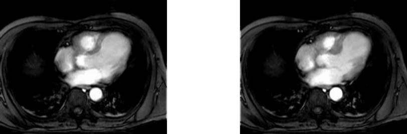
Figure 4.19 Query result of specific selection
Finally, this query calculates the sample variance of mr2:
select var_samp( mr2 ) from mr2
4.10.13. General Array Condenser
All condensers introduced previously are special cases of a general principle represented by the general condenser statement.
The general condense operation consolidates cell values of a multidimensional array to a scalar value based on the condensing operation indicated. It iterates over a spatial domain while combining the result values of the cellExps through the condenserOp indicated.
The general condense operation consolidates cell values of a multidimensional array to a scalar value or an array, based on the condensing operation indicated.
Condensers are heavily used in two situations:
To collapse boolean arrays into scalar boolean values so that they can be used in the where clause.
In conjunction with the marray constructor (see next section) to phrase high-level signal processing and statistical operations.
Syntax
condense condenserOp
over var in mintervalExp [ASC|DESC]
  [, var in mintervalExp [ASC|DESC] ]*
using cellExp

condense condenserOp
over var in mintervalExp [ASC|DESC]
  [, var in mintervalExp [ASC|DESC] ]*
where booleanExp
using cellExp
The mintervalExp terms together span a multidimensional spatial domain over which the condenser iterates. It visits each point in this space exactly once, assigns the point’s respective coordinates to the var variables and evaluates cellExp for the current point.
The result values are combined using condensing function condenserOp, which
can be one of +, or, and, max, min, or overlay.
Optionally, points used for the aggregate can be filtered through a
booleanExp; in this case, cellExp will be evaluated only for those
points where booleanExp is true, all others will not be regarded. Both
booleanExp and cellExp can contain occurrences of pointVar variables.
The cellExp is usually a scalar expression so that the result of the condense expression is a single scalar value, whether atomic or composite of several bands. Alternatively, it can also be an array-producing expression, in which case the condenserOp acts as an induced operation combining the arrays produced in each iteration; hence, this variant is also known as an induced condenser. It can be expressed with a combination of marray and scalar-producing condenser, but in most case the induced condenser will be clearer and execute more efficiently.
The order in which points in the spatial domain are visited is undefined, unless
ASC (ascending) or DESC (descending) is specified. Generally these are
not relevant as most operations are commutative and associative, so the order
does not influence the result; it only makes a difference if condenserOp is
overlay, which is not commutative.
Each condenserOp has an identity initial value of the condensed result. This
is the value that is returned when the booleanExp in the where clause filters
out all points so that cellExp in the using clause is never executed. For
+ and overlay this is 0, for max the smallest possible value
for the type of the cellExp and for min the largest, for and it is
true and for or it is false
Examples
This expression below returns a scalar representing the sum of all array
values, multiplied by 2 (effectively, this is equivalent to
add_cells(2*a)):
condense +
over x in sdom(a)
using 2 * a[ x ]
The following expression returns a 2-D array where cell values of 3-D array a are added up along the third axis:
condense +
over x in [0:100]
using a[ *:*, *:*, x[0] ]
Note that the addition is induced as the result type of the value clause is an array. This type of operation is frequent, for example, in satellite image time series analysis where aggregation is performed along the time axis.
Shorthands
Definition of the specialized condensers in terms of the general condenser statement is as shown in Table 4.5.
Aggregation definition |
Meaning |
|---|---|
add_cells(a) =
condense +
over x in sdom(a)
using a[x]
|
sum over all cells in a |
avg_cells(a) =
sum_cells(a) /
card(sdom(a))
|
Average of all cells in a |
min_cells(a) =
condense min
over x in sdom(a)
using a [x]
|
Minimum of all cells in a |
max_cells(a) =
condense max
over x in sdom(a)
using a[x]
|
Maximum of all cells in a |
count_cells(b) =
condense +
over x in sdom(b)
where b[x] != 0
using 1
|
Number of cells in b which are non-zero / not false |
some_cells(b) =
condense or
over x in sdom(b)
using b[x]
|
is there any cell in b with value true? |
all_cells(b) =
condense and
over x in sdom(b)
using b[x]
|
do all cells of b have value true? |
Restriction
Currently condensers over complex numbers are generally not supported, with
exception of add_cells and avg_cells.
4.10.14. General Array Constructor
The marray constructor allows to create n-dimensional arrays with their content defined by a general expression. This is useful
whenever the array is too large to be described as a constant (see Array Constants) or
when the array’s contents is derived from some other source, e.g., for a histogram computation (see examples below).
Syntax
The basic shape of the marray constructor is as follows:
marray var in mintervalExp
   [ , var in mintervalExp ]*
values cellExp
The cellExp describes how the resulting array is produced at each point of its spatial domain. It can be either a scalar-producing or an array-producing expression, a distinction that influences how the resulting array is constructed.
4.10.14.1. Scalar-producing Cell Expression
Here we consider the case when cellExp evaluates to a scalar, i.e., a single or composite value, as opposed to an array.
Iterator Variable Declaration
The result array is defined by the cross product of all mintervalExp. For example, the following defines a 2-D 5x10 matrix:
marray x in [1:5], y in [1:10]
values ...
The base type of the array is determined by the type of cellExp. Each variable var can be of any number of dimensions.
Iteration Expression
The resulting array is filled in at each coordinate of its spatial domain by successively evaluating cellExp; the result value is assigned to the cell at the coordinate currently under evaluation. To this end, cellExp can contain arbitrary occurrences of var, which are accordingly substituted with the values of the current coordinate. The syntax for using a variable is:
for a one-dimensional variable:
varfor a one- or higher-dimensional variable:
var [ index-expr ]
where index-expr is a constant expression evaluating to a non-negative integer; this number indicates the variable dimension to be used.
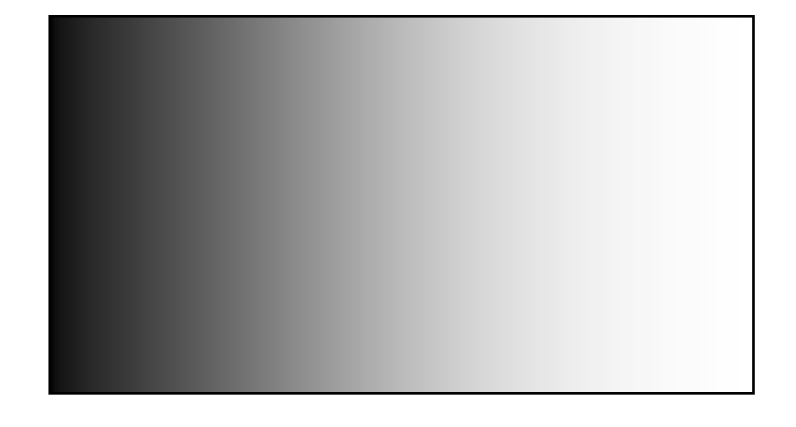
Figure 4.20 2-D array with values derived from first coordinate
Examples
The following creates an array with spatial domain [1:100,-50:200] over cell type char, each cell being initialized to 1.
marray x in [ 1:100, -50:200 ]
values 1c
In the next expression, cell values are dependent on the first coordinate component (cf. Figure 4.20):
marray x in [ 0:255, 0:100 ]
values x[0]
The final two examples comprise a typical marray/condenser combination. The first one takes a sales table and consolidates it from days to week per product. Table structure is as given in Figure 4.21.:
select marray tab in [ 0:sdom(s)[0].hi/7, sdom(s)[1] ]
       values condense +
              over day in [ 0:6 ]
              using s[ day[0] + tab7 ] , tab[1] ]
from salestable as s
The last example computes histograms for the mr images. The query creates a 1-D array ranging from 0 to 9 where each cell contains the number of pixels in the image having the respective intensity value.
select marray v in [ 0 : 9 ]
       values condense +
              over x in sdom(mr)
              where mr[x] = v[0]
              using 1
from mr

Figure 4.21 Sales table consolidation
4.10.14.2. Array-producing Cell Expression [RE]
The cellExp can alternatively evaluate to an array result:
marray var1 in mintervalExp, ...,
       varN in mintervalExp
values mddExp
In this case the result array is defined by the cross product of all mintervalExp, as well as the sdom of mddExp. For example, the following defines a 4-D 2x3x5x10 hypercube:
marray t in [1:2], h in [1:3]
values mr2[1:5, 1:10]
The variables var1 … varN can be used anywhere in the cell expression, as long as the expression remains valid in terms of the constraint defined later on.
This marray variant is in some sense equivalent to the following, where the cell expression is obviously a scalar-producing expression, as all dimensions of mddExp are sliced by sdomIter
marray var1 in mintervalExp, ...,
       varN in mintervalExp,
       sdomIter in sdom(mddExp)

values mddExp[sdomIter]
We say “in some sense”, because it is not possible to always practically rewrite it in this way, as mddExp could by a variable-bound expression that contains references to some of var1 … varN, and hence be invalid input for the sdom function. But it illustrates well how it works in principle, and due to the constraint defined below sdom(mddExpr) is fixed, so at least in theory it is valid.
Constraints
Let iteration domain be the cross product of all mintervalExp of var1 … varN. For each coordinate in the iteration domain, mddExp must evaluate to an array of the same spatial domain for it to be a valid cell expression. This allows to neatly place each result array slice of dimension D into the result of dimension N+D. Example of an invalid expression:
marray t in [0:2]
values B[0, 0:t]
Examples
Suppose we have a 3-D time-series array A; the goal is to select a 3-D subset out of it, such that each 2-D spatial slice is reprojected to a certain CRS:
marray t in [0:10]
values project( A[t, 0:1000, -50:2000], "EPSG:4326", ... )
The variable t iterates through the time axis coordinates of interest, and at each coordinate the 2-D slice is reprojected and placed into the resulting 3-D cube.
It is straightforward to do the opposite of dimension slicing: adding new dimensions to an array. E.g. to convert the 2-D array mr2 into a 3-D one:
MARRAY i in [0:0]
VALUES mr2
As mr2 has an sdom of [0:255,0:210], the result of the above expression has an sdom of [0:0,0:255,0:210]. It is essentially the same array, but now 3-dimensional. It may be useful in a case where the dimensionality of an array needs to be increased for some operation.
4.10.14.3. Common details
Shorthand
As a shorthand, variable var can be used without indexing; this is equivalent to var[0]:
marray x in [1:5]
values a[ x ]       -- equivalent to a[ x[0] ]
Many vs. One Variable
Obviously an expression containing several 1-D variables, such as:
marray x in [1:5], y in [1:10]
values a[ x[0], y[0] ]
can always be rewritten to an equivalent expression using one higher-dimensional variable, for example:
marray xy in [1:5, 1:10]
values a[ xy[0], xy[1] ]
Iteration Sequence Undefined
The sequence in which the array cells defined by an marray construct are inspected is not defined. In fact, server optimisation will heavily make use of reordering traversal sequence to achieve best performance.
A Note on Expressiveness and Performance
The general condenser and the array constructor together allow expressing a very broad range of signal processing and statistical operations. In fact, all other rasql array operations can be expressed through them, as Table 4.6 exemplifies. Nevertheless, it is advisable to use the specialized operations whenever possible; not only are they more handy and easier to read, but also internally their processing has been optimized so that they execute considerably faster than the general phrasing.
operation |
shorthand |
phrasing with marray |
|---|---|---|
Trimming |
a[ *:*, 50:100 ]
|
marray x in [sdom(a)[0], 50:100]
values a[ x ]
|
Section |
a[ 50, *:* ]
|
marray x in sdom(a)[1]
values a[ 50, x ]
|
Induction |
a + b
|
marray x in sdom(a)
values a[x] + b[x]
|
4.10.15. Type Coercion Rules
This section specifies the type coercion rules in query expressions, i.e. how the base type of the result from an operation applied on operands of various base types is derived.
The guiding design principle for these rules is to minimize the risk for overflow, but also “type inflation”: when a smaller result type is sufficient to represent all possible values of an operation, then it is preferred over a larger result type. This is especially important in the context of rasdaman, where the difference between float and double for example can be multiple GBs or TBs for large arrays. As such, the rules are somewhat different from C++ for example or even numpy, where in general careful explicit casting is required to avoid overflow or overtyping.
The type specifiers (c, o, s, …) are the literal type suffixes as documented
in Table 4.2; X and Y indicate any cell type,
U corresponds to any unsigned integer type, S to any signed integer
type, C to any complex type. In every table the upper rows have precedence,
i.e. the deduction rules are ordered; if a particular operand type combination
is missing it means that it is not supported and would lead to a type error. The
first/second operand types are commutative by default and only one direction is
shown to reduce clutter. Types have a rank determined by their size in bytes
and signedness, so that double has a higher rank than float, and long has higher
rank than ulong; max/min of two types returns the type with higher/lower type.
Adding 1 to a type results in the next type by rank, preserving signedness; the
integer/floating-point boundary is not crossed, however, i.e. long + 1 = long.
4.10.15.1. Binary Induced
Complex operands are only supported by +, -, \*, /, div, =, and !=. If any
operand of these operations is complex, then the result is complex with
underlying type derived by applying the rules to the underlying types of the
inputs. E.g. char + CInt16 = char + short = CInt32, and CInt32 * CFloat32
= long * float = CFloat64.
*
A special rule for multiplication applicable when one of the operands is boolean. In this case the result type does not change from the non-boolean operand.
first
second
result
X
bool
X
bool
X
X
+, *, div, mod
first
second
result
X
d
d
l,ul
f
d
X
f
f
U1
U2
max(U1, U2) + 1
X
Y
signed(max(X, Y) + 1)
- (subtraction)
The result can always be negative, even if inputs are unsigned (positive), so for integers the result type is always the next greater signed type. Otherwise, the rules are the same as for +, *, div, mod.
first
second
result
X
d
d
l,ul
f
d
X
f
f
X
Y
signed(max(X, Y) + 1)
/ (division)
Division returns floating-point to avoid inadvertent precision loss as well as
unnecessary check for division by zero. Integer division is supported with the
div function.
first
second
result
c,o,s,us,f
c,o,s,us,f
f
X
Y
d
pow, power
Note: operand types are not commutative, the second operand must be a float or double scalar.
first
second
result
c,o,s,us,f
c, o, s, us, f
f
ul,l,d
f, d
d
arctan2
first
second
result
f
f
f
d
d
d
<, >, <=, >=, =, !=
first
second
result
X
Y
bool
min, max, overlay
first
second
result
X
X
X
and, or, xor, is
first
second
result
bool
bool
bool
bit
I stands for any signed and unsigned integer type.
The second operand must be a positive value, i.e. an unsigned integer type.
first
second
result
I
c,us,ul
bool
complex(re, im)
first (re)
second (im)
result
s
s
CInt16
l
l
CInt32
f
f
CFloat32
d
d
CFloat64
4.10.15.2. Unary Induced
not
op
result
bool
bool
abs
op
result
C
error
X
X
sqrt, log, ln, exp, sin, cos, tan, sinh, cosh, tanh, arcsin, arccos, arctan
op
result
c,o,us,s,f
f
u,l,d
d
ceil, floor, round
op
result
X
X
4.10.15.3. Condensers
count_cells
op
result
bool
ul
add_cells and condense +, *
op
result
C
CFloat64
f,d
d
S
l
U
ul
avg_cells
op
result
C
CFloat64
X
d
stddev_pop, stddev_samp, var_pop, var_samp
op
result
C
error
X
d
min_cells, max_cells and condense min, max
op
result
C
error
X
X
some_cells, all_cells and condense and, or
op
result
bool
bool
4.10.15.4. Geometric Operations
The base type does not change in the result of subset, shift, extend, scale, clip, concat, and geographic reprojection.
op
result
X
X
4.10.16. Polygonize operation
The polygonize function creates vector polygons for all connected regions of
pixels in a given array, resulting in a vector format file such as Shapefile.
This operation is useful in geographical context, providing ability to layer
additional information on existing maps, for example.
Syntax
polygonize(mddExp, targetFormat)
polygonize(mddExp, targetFormat, connectedness)

polygonize(mddExp, targetFormat, crs, bbox)
polygonize(mddExp, targetFormat, connectedness, crs, bbox)
Where
targetFormat: StringLit
connectedness: integerLit

crs: StringLit
bbox: StringLit
The targetFormat indicates the vector file format in which the result will
be encoded. To check supported targetFormat, refer to the GDAL
documentation. Only those
formats can be used that support creation option.
The connectedness parameter can be set to 4 or 8; if omitted, it will be set
to 4 by default. Setting it to 4 would ensure a ‘true’-cell can only be
considered a neighbor if it shares at least a corner with some
other ‘true’-cell. If we set the connectedness parameter to 8, a ‘true’-cell
can only be a neighbor if it shares a least an edge with some
other ‘true’-cell.
The crs is the geographic CRS of the mddExp. The same CRS formats as GDAL are accepted:
Well Known Text (as per GDAL)
“EPSG:n”
“EPSGA:n”
“AUTO:proj_id,unit_id,lon0,lat0” indicating OGC WMS auto projections
“urn:ogc:def:crs:EPSG::n” indicating OGC URNs (deprecated by OGC)
PROJ.4 definitions
well known names, such as NAD27, NAD83, WGS84 or WGS72.
WKT in ESRI format, prefixed with “ESRI::”
“IGNF:xxx” and “+init=IGNF:xxx”, etc.
Since recently (v1.10), GDAL also supports OGC CRS URLs, OGC’s preferred way of identifying CRSs.
The bbox parameter is a geographic bounding box given as a string of
comma-separated floating-point values of the format: “xmin, ymin, xmax, ymax”.
As a result, the operation produces a file in the desired target format. If the format results in several output files, they will be packaged in a zip archive.
Limitations
The implementation uses GDALPolygonize internally, so it has similar limitations. In particular, arrays with complex values are not supported, and floating-point arrays will be truncated to 64-bit integer. The operation is applicable only on single-band 2-D arrays.
Examples
The following query uses default parameters to polygonize rgb collection:
select polygonize(rgb) from rgb
The result is a .zip archive that consists of the three files in accordance
to the “ESRI Shapefile” format: polygonize.shp, polygonize.shx,
polygonize.dbf
The next query produces the result in pdf format:
select polygonize(rgb, "PDF") from rgb
The retrieved file is polygonize.pdf.
To specify 8-connectedness instead of the default 4, one can use the following query:
select polygonize(rgb, "ESRI Shapefile", 8) from rgb
If the input array is geo-referenced, its CRS and geo bbox can be specified:
select polygonize(c, "EPSG:4326", "-180, -90, 180, 90") from worldmap as c
4.11. Data Import
The decode() function allows for decoding data represented in one of
the supported formats, into an MDD which can be persisted or processed in
rasdaman.
4.11.1. Syntax
decode( mddExp )

encode( mddExp , format , formatParameters )
As a first paramater the data to be decoded must be specified. Technically this
data must be in the form of a 1D char array. Usually it is specified as a query
input parameter with $1, while the binary data is attached with the
--file option of the rasql command-line client tool, or with the
corresponding methods in the client API. If the data is on the same machine as
rasdaman, it can be loaded directly by specifying the path to it in the format
parameters; more details on this in Format parameters.
4.11.2. Data format
The source data format is automatically detected in case it is handled by GDAL
(e.g. PNG, TIFF, JPEG, etc; see output of gdalinfo --formats or the GDAL
documentation for a full list),
so there is no format parameter in this case.
A format is necessary, however, when a custom internal implementation should be
selected instead of GDAL for decoding the data, e.g. NetCDF ("netcdf" /
"application/netcdf"), GRIB ("grib"), JSON ("json" /
"application/json"), or CSV ("csv" / "text/csv").
4.11.3. Format parameters
Optionally, a format parameters string can be specified as a third parameter,
which allows to control the format decoding. For GDAL formats it is necessary to
specify format "GDAL" in this case.
The format parameters must be formatted as a valid JSON object. As the format
parameters are in quotes, i.e. "formatParameters", all quotes inside of the
formatParameters need to be escaped (\"). For example,
"{ \"transpose\": [0,1] }" is the right way to specify transposition, while
"{ "transpose": [0,1] }" will lead to failure. Note that in examples further
on quotes are not escaped for readability.
The following parameters are common to GDAL, NetCDF, and GRIB data formats:
variables- An array of variable names or band ids (0-based, as strings) to be extracted from the data. This allows to decode only some of the variables in a NetCDF file for example with["var1", "var2"], or the bands of a TIFF file with["0", "2"].filePaths- An array of absolute paths to input files to be decoded, e.g.["/path/to/rgb.tif"]. This improves ingestion performance if the data is on the same machine as the rasdaman server, as the network transport is bypassed and the data is read directly from disk. Supported only for GDAL, NetCDF, and GRIB data formats.Note that the system user running the rasserver processes must have read permissions on the specified files.
subsetDomain- Specify a subset to be extracted from the input file, instead of the full data. The subset should be specified in rasdaman minterval format as a string, e.g."[0:100,0:100]". Note that the subset domain must match in dimensionality with the file dimensionality, and must be accordingly offset to the grid origin in the file, which is typically [0,0,0,…].transpose- Specify if x/y should be transposed with an array of 0-based axis ids indicating the axes that need to be transposed; the axes must be contiguous[N,N+1], e.g.[0,1]. This is often relevant in NetCDF and GRIB data which have a swapped x/y order than what is usually expected in e.g. GDAL. Note that transposing axes has a performance penalty, so avoid if possible.formatParameters- A JSON object containing extra options which are format-specific, specified as string key-value pairs. This is where one would specify the base type and domain for decoding a CSV file for example, or GDAL format-specific options. Example for a CSV file:"formatParameters": { "basetype": "struct { float f, long l }", "domain": "[0:100,0:100]" }
4.11.4. 2D image formats
2D image formats are decoded with the GDAL library into the internal format of rasdaman. Besides the Format parameters, additionally the following format parameters are supported:
formatParameters- any entries in the formatParameters object are forwarded to the specific GDAL driver; consult the GDAL documentation for the options recognized by each particular driver. E.g. for PNG you could specify, among other details, a description metadata field with:"formatParameters": { "DESCRIPTION": "Data description..." }
configOptions- A JSON object containing configuration options as string key-value pairs; more details in the GDAL documentation. Example:"configOptions": { "GDAL_CACHEMAX": "64", ... }
openOptions- A JSON object containing open options as string key-value pairs; an option for selecting overview level from the file with, e.g."OVERVIEW_LEVEL": "2", is available for all formats (more details); further options may be supported by each driver, e.g. for TIFF;"openOptions": { "OVERVIEW_LEVEL": "2", "NUM_THREADS": "ALL_CPUS" }
Note
This feature is only available since GDAL 2.0, so if you have an older GDAL these options will be ignored.
4.11.4.1. Examples
The following query loads a TIFF image into collection
rgb:rasql -q 'insert into rgb values decode( $1 )' --file rgb.tif
If you use double quotes for the query string, note that the
$must be escaped to avoid interpretation by the shell:rasql -q "insert into rgb values decode( \$1 )" --file rgb.tif
The example below shows directly specifying a file path in the format parameters;
<[0:0] 1c>is a dummy array value which is not relevant in this case, but is nevertheless mandatory:UPDATE test_mr SET test_mr[0:255,0:210] ASSIGN decode(<[0:0] 1c>, "GDAL", "{ \"filePaths\": [\"/home/rasdaman/mr_1.png\"] }") WHERE oid(test_mr) = 6145
4.11.5. GRIB
internalStructure- Describe the internal structure of a GRIB file, namely the domains of all messages to be extracted from the file:"internalStructure": { "messageDomains": [ { "msgId": 1, "domain": "[0:0,0:0,0:719,0:360]" }, { "msgId": 2, "domain": "[0:0,1:1,0:719,0:360]" }, { "msgId": 3, "domain": "[0:0,2:2,0:719,0:360]" }, ... ] }
4.11.6. CSV / JSON
The following are mandatory options that have to be specified in the
formatParameters object when decoding CSV or JSON data:
domain- The domain of the MDD encoded in the CSV data. It has to match the number of cells read from input file, e.g. for"domain": "[1:5, 0:10, 2:3]", there should be 110 numbers in the input file.basetype- Atomic or struct base type of the cell values in the CSV data; named structs likeRGBPixelare not supported. Examples:long char struct { char red, char blue, char green }
Numbers from the input file are read in order of appearance and stored without any reordering in rasdaman; whitespace plus the following characters are ignored:
'{', '}', ',', '"', '\'', '(', ')', '[', ']'
4.11.6.1. Examples
Let array
Abe a 2x3 array of longs given as a string as follows:1,2,3,2,1,3
Inserting
Ainto rasdaman can be done withinsert into A values decode($1, "csv", "{ \"formatParameters\": { \"domain\": \"[0:1,0:2]\", \"basetype\": \"long\" } }")
Let
Bbe an 1x2 array of RGB values given as follows:{1,2,3},{2,1,3}
Inserting
Binto rasdaman can be done by passing it to this query:insert into B values decode($1, "csv", "{ \"formatParameters\": { \"domain\": \"[0:0,0:1]\", \"basetype\": \"struct{char red, char blue, char green}\" } }")
Bcould just as well be formatted like this with the same effect (note the line break):1,2,3 2,1,3
4.12. Data Export
The encode() function allows encoding an MDD in a particular data format
representation, such as TIFF, PNG, NetCDF, JSON, CSV, etc.
Formally, the result returned by the rasdaman server will be a 1D char (byte)
array.
4.12.1. Syntax
encode( mddExp , format )

encode( mddExp , format , formatParameters )
The first parameter is the MDD to be encoded. It must be 2D if encoded to GDAL formats (PNG, TIFF, JPEG, etc.), while the native rasdaman encoders (NetCDF, JSON, and CSV) support MDDs of any dimension. Note that presently encode to GRIB is not supported. As not all base types supported by rasdaman (char, octet, float, etc.) are necessarily supported by each format, care must be taken to cast the MDD beforehand.
4.12.2. Data format
A mandatory format must be specified as the second parameter, indicating
the data format to which the MDD will be encoded; allowed values are
GDAL format identifiers (see output of
gdalinfo --formatsor the GDAL documentation);a mime-type string, e.g.
"image/png";"netcdf"/"application/netcdf","csv"/"text/csv", or"json"/"application/json", for formats natively supported by rasdaman.
4.12.3. Format parameters
Optionally, a format parameters string can be specified as a third parameter,
which allows to control the format encoding. As in the case of decode(), it must
be a valid JSON object. As the format parameters are in quotes, i.e.
"formatParameters", all quotes inside of the formatParameters need to be
escaped (\"). For example, "{ \"transpose\": [0,1] }" is the right way
to specify transposition, while "{ "transpose": [0,1] }" will lead to
failure due to the nested double quotes.
Common parameters to most or all formats include:
metadata- A single string, or an object of string key-value pairs which are added as global metadata when encoding.transpose- Specify if x/y should be transposed with an array of 0-based axis ids indicating the axes that need to be transposed; the axes must be contiguous[N,N+1], e.g.[0,1]. This is often relevant when encoding data with GDAL formats, which was originally imported from NetCDF and GRIB files. Note that transposing axes has a performance penalty, so avoid if possible.nodata- Specify nodata value(s). If a single number is specified it will be applicable to all bands (e.g.0), otherwise an array of numbers for each band can be provided (e.g.[0,255,255]). Special floating-point constants are supported (case-sensitive): NaN, NaNf, Infinity, -Infinity.formatParameters- A JSON object containing extra options which are format-specific, specified as string key-value pairs. This is where one would specify the options for controling what separators and values are used in CSV encoding for example, or GDAL format-specific options.
4.12.4. 2D image formats
Arrays in rasdaman are encoded into 2D image formats with the GDAL library. Besides the Format parameters, additionally the following format parameters are supported:
formatParameters- any entries in the formatParameters object are forwarded to the specific GDAL driver; consult the GDAL documentation for the options recognized by each particular driver. E.g. for PNG you could specify, among other details, a description metadata field with:"formatParameters": { "DESCRIPTION": "Data description..." }
Rasdaman itself does not change the default values for these parameters, with the following exceptions:
PNG- the compression level when encoding to PNG (optionZLEVEL) will be set to2if the user does not specify it explicitly and the result array is not of typeboolean. The default compression level of6does not offer considerable space savings on typical image results (e.g. around 10% lower file size for satellite image), while significantly increasing the time to encode, taking up to 3-5x longer.
configOptions- A JSON object containing configuration options as string key-value pairs; only relevant for GDAL currently, more details in the GDAL documentation. Example:"configOptions": { "GDAL_CACHEMAX": "64", ... }
4.12.4.1. Geo-referencing
geoReference- An object specifying geo-referencing information; either “bbox” or “GCPs” must be provided, along with the “crs”:crs- Coordinate Reference System (CRS) in which the coordinates are expressed. Any of the CRS representations acceptable by GDAL can be used:Well known names, such as
"NAD27","NAD83","WGS84"or"WGS72""EPSG:n","EPSGA:n"PROJ.4 definitions
OpenGIS Well Known Text
ESRI Well Known Text, prefixed with
"ESRI::"Spatial References from URLs
"AUTO:proj_id,unit_id,lon0,lat0"indicating OGC WMS auto projections"urn:ogc:def:crs:EPSG::n"indicating OGC URNs (deprecated by OGC)
bbox- A geographic X/Y bounding box as an object listing the coordinate values (as floating-point numbers) forxmin,ymin,xmax, andymaxproperties, e.g.:"bbox": { "xmin": 0.0, "ymin": -1.0, "xmax": 1.0, "ymax": 2.0 }
GCPs- Alternative to abbox, an array of GCPs (Ground Control Points) can be specified; see GCPs section in the GDAL documentation for details. Each element of the array is an object describing one control point with the following properties:id- optional unique identifier (gets the GCP array index by default);info- optional text associated with the GCP;pixel,line- location on the array grid;x,y,z- georeferenced location with coordinates in the specified CRS; “z” is optional (zero by default);
4.12.4.2. Coloring Arrays
colorMap- Map single-band cell values into 1, 3, or 4-band values. It can be done in different ways depending on the specified type:values- Each pixel is replaced by the entry in thecolorTablewhere the key is the pixel value. In the example below, it means that all pixels with value -1 are replaced by [255, 255, 255, 0]. Pixels with values not present in the colorTable are not rendered: they are replaced with a color having all components set to 0."colorMap": { "type": "values", "colorTable": { "-1": [255, 255, 255, 0], "-0.5": [125, 125, 125, 255], "1": [0, 0, 0, 255] } }
intervals- All pixels with values between two consecutive entries are rendered using the color of the first (lower-value) entry. Pixels with values equal to or less than the minimum value are rendered with the bottom color (and opacity). Pixels with values equal to or greater than the maximum value are rendered with the top color and opacity."colorMap": { "type": "intervals", "colorTable": { "-1": [255, 255, 255, 0], "-0.5": [125, 125, 125, 255], "1": [0, 0, 0, 255] } }
In this case, all pixels with values in the interval (-inf, -0.5) are replaced with [255, 255, 255, 0], pixels in the interval [-0.5, 1) are replaced with [125, 125, 125, 255], and pixels with value >= 1 are replaced with [0, 0, 0, 255].
ramp- Same as “intervals”, but instead of using the color of the lowest value entry, linear interpolation between the lowest value entry and highest value entry, based on the pixel value, is performed."colorMap": { "type": "ramp", "colorTable": { "-1": [255, 255, 255, 0], "-0.5": [125, 125, 125, 255], "1": [0, 0, 0, 255] } }
Pixels with value -0.75 are replaced with color [189, 189, 189, 127], because they sit in the middle of the distance between -1 and -0.5, so they get, on each channel, the color value in the middle. The interpolation formula for a pixel of value x, where 2 consecutive entries in the colorTable \(a, b\) with \(a \le x \le b\), is:
\[resultColor = \frac{b - x}{b - a} * colorTable[a] + \frac{x - a}{b - a} * colorTable[b]\]For the example above, a = -1, x = -0.75, b = -0.5, colorTable[a] = [255, 255, 255, 0], colorTable[b] = [125, 125, 125, 255], so:
\[\begin{split}resultColor &= \frac{-0.5 + 0.75}{-0.5 + 1} * [255, 255, 255, 0] + \\ & \hspace{1.5em} \frac{-0.75 + 1}{-0.5 + 1} * [125, 125, 125, 255] \\ &= 0.5 * [255, 255, 255, 0] + 0.5 * [125, 125, 125, 255] \\ &= [127, 127, 127, 0] + [62, 62, 62, 127] \\ &= [189, 189, 189, 127] \\\end{split}\]Note the integer division, because the colors are of type unsigned char.
colorPalette- Similar tocolorMap, however, it allows specifying color information on a metadata level, rather than by actually transforming array pixel values; for details see the GDAL documentation. It is an object that contains several optional properties:paletteInterp- Indicate how the entries in the colorTable should be interpreted; allowed values are “Gray”, “RGB”, “CMYK”, “HSL” (default “RGB”);colorInterp- Array of color interpretations for each band; allowed values are Undefined, Gray, Palette, Red, Green, Blue, Alpha, Hue, Saturation, Lightness, Cyan, Magenta, Yellow, Black, YCbCr_Y, YCbCr_Cb, YCbCr_Cr, YCbCr_Cr;colorTable- Array of arrays, each containing 1, 3, or 4 short values (depending on thecolorInterp) for each color entry; to associate a color with an array cell value, the cell value is used as a subscript into the color table (starting from 0).
4.12.4.3. Examples
This query extracts PNG images (one for each tuple) from collection mr:
select encode( mr, "png" )
from mr
Transpose the last two axes of the output before encoding to PNG:
select encode(c, "png", "{ \"transpose\": [0,1] }") from mr2 as c
4.12.5. NetCDF
The following are mandatory options when encoding to NetCDF:
dimensions- An array of names for each dimension, e.g.["Lat","Long"].variables- Specify variable names for each band of the MDD, dimension names if they need to be saved as coordinate variables, as well as non-data grid mapping variables. There are three ways to specify the variables:An array of strings for each variable name, e.g.
["var1", "var2"]; no coordinate variables should be specified in this case, as there is no way to specify the data for them;An array of variable objects, where each object lists the following variable details:
name- The variable name, e.g."name": "var1"metadata- An object of string key-value pairs which are added as attributes to the variable;type- Type of the data values this variable contains relevant (and required) for coordinate or non-data variables; allowed values are “byte”, “char”, “short”, “ushort”, “int”, “uint”, “float”, and “double”;data- An array of data values for the variable relevant (and required) only for coordinate variables (as regular variables get their data values from the array to be encoded); the number of values must match the dimension extent;
If the variable name is not listed in the
dimensionsarray and still has adataattribute, then it will be considered to be a non-data variable and will not be used for storing MDD band data; thedataattribute is ignored in this case, so the value for it can be an empty JSON array[].An object of variable name - object pairs, where each object lists the variable details in similar fashion to the option 2. above, except that the key
nameis optional. This way of specifying the variables in a JSON object is deprecated because their order is non-deterministic and may not work as expected when encoding multiple variables. It is recommended to use the method in option 2.
4.12.5.1. Examples
Add some global attributes as metadata in netcdf:
select encode(c, "netcdf", "{ \"transpose\": [1,0], \"nodata\": [100],
    \"metadata\": { \"new_metadata\": \"This is a new added metadata\" } }")
from test_mean_summer_airtemp as c
The format parameters below specify the variables to be encoded in the result NetCDF file (Lat, Long, forecast, and drought_code); of these Lat, Long, and forecast are dimension variables for which the values are specified in the
"data"array, which leaves drought_code is the proper variable for encoding the array data.Below format parameters for a rotated grid are specified, which define a
"rotated_pole"grid mapping variable in addition to the dimension variables (rlongandrlat) and the band variableCAPE_ML. More information on grid mappings can be found here.
4.12.6. CSV / JSON
Data encoded with CSV or JSON is a comma-separated list of values. By default the cell values are linearized in row-major order where the last dimension of the array’s spatial domain iterates fastest while serializing the values.
JSON is recommended as it results in a well-defined JSON string that can be
parsed with any JSON library. Null values are clearly distinguished with the
standard null keyword.
CSV works well for 2-D arrays where by default each column (the last dimension of the array’s spatial domain) is encoded as one row on a separate line. If the array’s dimension is greater than 2, then 2-D slices in the output are separated by a single empty line, multiple 2-D slices comprising a single 3-D slice are separated by two empty lines, and so on. Null values are encoded as an empty string by default.
In both cases, composite values are encoded as space-separated component values
enquoted in double quotes, e.g. "0 128 255". Nulls within the enquoted
value are encoded in the same fashion as for atomic values: null for JSON
(e.g. "null 128 255") or an empty string for CSV (e.g. " 128 255").
The table below documents all “formatParameters” options that allow controlling the output, and the default settings for both formats.
option |
description |
CSV default |
JSON default |
|---|---|---|---|
|
array linearization order, can be “outer_inner” (default, last dimension iterates fastest, i.e. row-major for 2-D), or vice-versa, “inner_outer”. |
“outer_inner” |
“outer_inner” |
|
serialize null values as nullValue if true |
true |
true |
|
string denoting null values (if enableNull is true) |
“” |
“null” |
|
string denoting true values |
“t” |
“true” |
|
string denoting false values |
“f” |
“false” |
|
string to indicate starting a new dimension slice |
“” |
“[” |
|
string to indicate ending a dimension slice |
“” |
“]” |
|
separator between dimension slices |
“n” |
“,” |
|
separator between cell values |
“,” |
“,” |
|
separator between components of struct cell values |
“ “ |
“ “ |
|
string to indicate starting a new struct value |
“\"” |
“\"” |
|
string to indicate ending a new struct value |
“\"” |
“\"” |
|
wrap output in dimensionStart and dimensionEnd |
false |
true |
|
encode each 1-D slices on a new line and indent JSON |
true |
true |
4.12.6.1. Examples
Suppose we have array A = <[0:1,0:1] 0, 1; 2, 3>.
Encoding to CSV by default with
select encode(A, "csv") from A
will result in the following output:
0,1
2,3
Encoding to JSON with
select encode(A, "json") from A
will result in the following output:
[
 [0,1],
 [2,3]
]
Specifying
inner_outerorder with:select encode(A, "csv", "{ \"formatParameters\": { \"order\": \"inner_outer\" } }") from A
will result in the following output (left-most dimensions iterate fastest):
0,2
1,3
Let
Bbe an RGB array<[0:0,0:1] {0c, 1c, 2c}, {3c, 4c, 5c}>. Encoding it to CSV with default order will result in the following output:"0 1 2","3 4 5"
4.13. Object identifiers
Function oid() gives access to an array’s object identifier (OID). It
returns the local OID of the database array. The input parameter must be
a variable associated with a collection, it cannot be an array
expression. The reason is that oid() can be applied to only to
persistent arrays which are stored in the database; it cannot be applied
to query result arrays - these are not stored in the database, hence do
not have an OID.
Syntax
oid( variable )
Example
The following example retrieves the MDD object with local OID 10 of set
mr:
select mr
from mr
where oid( mr ) = 10
The following example is incorrect as it tries to get an OID from a non-persistent result array:
select oid( mr * 2 ) -- illegal example: no expressions
from mr
Fully specified external OIDs are inserted as strings surrounded by brackets:
select mr
from mr
where oid( mr ) = < localhost | RASBASE | 10 >
In that case, the specified system (system name where the database server runs) and database must match the one used at query execution time, otherwise query execution will result in an error.
4.13.1. Expressions
Parentheses
All operators, constructors, and functions can be nested arbitrarily, provided that each sub-expression’s result type matches the required type at the position where the sub-expression occurs. This holds without limitation for all arithmetic, Boolean, and array-valued expressions. Parentheses can (and should) be used freely if a particular desired evaluation precedence is needed which does not follow the normal left-to-right precedence.
Example
select (rgb.red + rgb.green + rgb.blue) / 3c
from rgb
Operator Precedence Rules
Sometimes the evaluation sequence of expressions is ambiguous, and the different evaluation alternatives have differing results. To resolve this, a set of precedence rules is defined. You will find out that whenever operators have their counterpart in programming languages, the rasdaman precedence rules follow the same rules as are usual there.
Here the list of operators in descending strength of binding:
dot “.”, trimming, section
unary
-sqrt,sin,cos, and other unary arithmetic functions*,/+,-<,<=,>,>=,!=,=andor,xor“:” (interval constructor),
condense,marrayoverlay,concatIn all remaining cases evaluation is done left to right.
4.14. Null Values
This section introduces handling of null values in queries. Type definition of null values is explained in Set types.
4.14.1. Introduction
Null is a special marker commonly used in databases to indicate non-existing data values. In rasdaman, it means that in some array cell there is no value that can be used for anything. A variety of reasons exist for such missing values: a sensor detected an erroneous reading, no value was provided at all (maybe due to transmission problems), no values are applicable to this position at all (such as sea surface temperature measurements on dry land positions), etc. As arrays by definition have a value for every position inside the array spatial domain, a “placeholder” must exist which reserves the place (thereby not disturbing array order) while indicating that the value is not to be used. We call such cells null values.
In rasdaman two ways exist to model null values:
by keeping a flag (called “null flag” or “null mask”) for each cell indicating whether it is null or not; this is the common approach in databases;
by designating one or more of the possible values of a cell as representing a null value; we call the set of these possible values the “null set”; this is the common way of representing nulls in sensor data acquisition.
Starting with version 10.0 both methods are supported by rasdaman in a compatible manner. The null set is important for compatibility with sensor data encoded in various formats, while the null mask is crucial for producing accurate results during query processing.
Null masks will propagate through all operations into the result. Hence the result of every sub-expression will have a null mask, even if it is an ‘’empty mask’’ (indicating that all array cells are valid). Null masks influence the behavior of most operations as elaborated further on.
Null sets on the other hand will generally not be propagated, except in operations that do not change the cell values of an array, such as subsetting, clip(), project(), etc. This is so because the result of an operation, such as addition, may suddenly contain cell values that are in the null set, even if they were not originally so in the operands of this operation.
In the operations considered below it is always explicitly mentioned when the null set is propagated. While the null set may be propagated by operations, it may only have an effect when loading an array from disk with associated null values, explicitly setting a null set to the result of an array expression, or encoding an array to some data format.
Both null mask and null set are per-band in the case of multi-band arrays. It is not possible to associate a single null mask to multiple bands at once so that it indicates that a composite pixel as a whole is null.
4.14.2. Persisting data
The insert and update statements allow persisting array data into the database.
An array A to be newly inserted or updated, must match the type of the collection into which it is being persisted. Besides the base type and dimension, the following rules are additionally in place for validating that the null set S of A matches the null set S’ of the target collection:
if S is empty, then the array can be inserted/updated regardless of S’; this is allowed to avoid a common issue where decoded arrays do not get a nullset automatically from the data, due to no support by the format for example.
otherwise, if S is not equal to S’ then an error is thrown.
Persisting of null masks is not supported, so if A has a null mask it will be discarded.
Note
Presently these rules are not enforced, but will likely be in future.
4.14.3. Loading data
When loading arrays from the database during query evaluation, the null set if present is attached to the loaded array. How null masks are handled at this stage depends on whether data was imported or registered.
If an array was imported
if null sets are present, then they are applied to the data to generate a null mask for each band;
otherwise, the array will have no null mask associated.
If an array was registered and does not get a null mask associated according to the above rules for imported data, then a null mask may still be attached if
the encoded data contains null masks (for GDAL formats), or
the encoded data contains null values, which are applied on the data after decoding to create null masks for each band (GDAL/NetCDF formats)
In both cases, the resulting array object will have (possibly empty) null masks associated and (possibly empty) null sets.
4.14.4. Array constructor
If evaluation of the values clause for some cell accesses an array with null
masks, then the result of evaluating the expression will have null masks; the
mask’s null flag for each cell of the new array is determined depending on the
operations involved in the values expression. Otherwise, the new array will
have an empty null mask, with all flags reset to false.
The detail behavior of operations derived from array constructor is as follows:
operation |
null value behavior |
|---|---|
range constructor |
null status of the record components remain unchanged |
band selection |
null status of the selected band remains unchanged |
subsetting |
each cell and its null status remain unchanged |
shift |
null status of the operand remains unchanged |
extend |
will set new cells to null, and will not change existing cells or their null status |
scale |
will scale both data and operand null mask with the same algorithm |
concat |
1) create a null mask for the result if any of the operands has one; 2) initialize the null mask to false (i.e., not null) for all cells; 3) copy over null masks from the operands having null masks into the result, at the appropriate target coordinate in the concatenated array. |
induced operations |
the result has null mask only if some operand has a null mask; if at least one cell operand is null then the result cell will be null, too |
If the operand has a null set, then it will be propagated to the result as is through range constructor, struct selection, subsetting, shift, extend, and scale.
4.14.5. Array clipping
The clip() function always results in a null mask along with the result array.
cells outside the clipped region are set to null
cells inside the clipped region along with their null status remain unchanged
If the operand has a null set then it will be propagated to the result as is.
4.14.6. Array reprojection
The project() function always results in a null mask along with the result array.
if the input has a null mask then it is reprojected in the same way as the array
otherwise, a new null mask is generated and set to true for cells outside the original array data
If the operand has a null set then it will be propagated to the result as is.
4.14.7. Array aggregation
Cell values which are null according to the null mask, if it exists, are ignored in the general condenser and shorthands (add_cells, count_cells, etc).
If all cells are null or a where clause returns false in all cases, then the result is a scalar null.
4.14.8. Null-specific operators
4.14.8.1. Dynamically changing null values
mddExp null values nullClause allows to explicitly set a null set to mddExp.
The nullClause must conform to the same syntax and semantics rules for type
definition as in Set types. If mddExp already has a null set it will
be overwritten with the newly specified one.
mddExp null values nullset(mddExp2) is same as above, except that the null
set is copied from mddExp2, rather than explicitly specified.
In both cases, a new null mask will be generated for mddExp from the newly specified null set.
4.14.8.2. Dynamically changing null masks
mddExp null mask boolMddExp allows to explicitly set a null mask to mddExp.
The spatial domains of mddExp and boolMddExp must be matching as in the case of
binary operations. If mddExp is multi-band then the same boolMddExp mask will be
set to all bands. If mddExp already has a null mask it will be overwritten with
boolMddExp.
mddExp null mask discard allows to remove the null mask from mddExp. It has
no effect if the mddExp has no null mask.
4.14.8.3. Retrieving the null mask
X is null (postfix) returns the null mask of X, a boolean array with domain
sdom(X). X must be single band, otherwise an error is thrown.
4.14.8.4. Retrieving the null set
nullset(X) returns the null set of X as a string.
4.14.9. Encoding data
Let A be the array to be encoded with base type BT, and M the null mask of A. Let NV be the value of parameter “nodata” in the format parameters of encode() if specified, otherwise a random value from the null set of A if available (lower or upper bound in case of a null value interval).
Data format support for encoding null values varies.
4.14.9.1. GDAL formats (TIFF, JPEG, PNG, etc)
The band nodata value will be set to NV if available.
If a 4-band color map (with transparency) is specified in the format parameters,
then the array to be encoded is first transformed according to the color map.
Let TV be the first transparent pixel in the color table if one is specified, or
[0,0,0,0] otherwise. All cell values which are null are set to TV in the
color mapped result.
4.14.9.2. NetCDF
Let FV be NV if NV is set, otherwise, if the array has a non-empty null mask then let FV be a default value according to BT (see NetCDF’s defaults):
base type BT
default null value NV
octet
-127
short
-32767
long
-2147483647
char
255
ushort
65535
ulong
4294967295
float
9.9692099683868690e+36
double
9.9692099683868690e+36
When encoding to NetCDF the _FillValue and missing_value attributes of
the output variables are set to FV. All cell values that are null according to
the null mask are set to FV, before encoding. M is discarded as NetCDF has no
support/convention for null masks.
4.14.9.3. JSON
Cell values that are null according to the null mask are encoded as “null” in
the output, e.g. [1, null, null, 100].
4.14.9.4. CSV
Cell values that are null according to the null mask are encoded as any other cell value without any changes. Hence their value is undefined, as operation may or may not have changed them during processing.
4.14.10. Decoding data
A decode operation may be able to extract null set or null mask from the
encoded data, depending on the particular format, and associate them with the
decoded array. Additionally, they can be explicitly set as for any other mddExp
(see Null-specific operators).
If a null set is extracted from the input data but not a mask, then a null mask is immediately generated for each band.
4.14.10.1. GDAL formats (TIFF, JPEG, PNG, etc)
The null set is collected from the nodata values of each band, and the null masks from the input nodata masks.
4.14.10.2. NetCDF
The null set is collected from the _FillValue and missing_value
attributes of the input variable if present.
4.14.10.3. CSV / JSON
There is no way to collect null set or null mask from these files. They can be always set dynamically however, see Null-specific operators.
4.14.11. NaN Values
NaN (“not a number”) is the representation of a numeric value representing an undefined or unrepresentable value, especially in floating-point calculations. Systematic use of NaNs was introduced by the IEEE 754 floating-point standard (Wikipedia).
In rasql, nan (double) and nanf (float) are symbolic floating point
constants that can be used in any place where a floating point value is allowed.
Arithmetic operations involving nans always result in nan. Equality
and inequality involving nans work as expected, all other comparison operators
return false.
If the encoding format used supports NaN then rasdaman will encode/decode NaN values properly.
Example
select count_cells( c != nan ) from c
4.14.12. Examples
The examples below illustrate null value behavior.
4.14.12.1. Example 1
Let A be a 2-D array <[1:1,1:2] 0c, 1c>, and GreySetNullValues a set type
defined as
-- values equal to 0 in the array are null values
create type GreySetNullValues
as set ( GreyImage null values [0] )
The bellow will insert A into a collection of the above type; this is allowed as A’s null set is empty.
insert into CollGreySetNullValues
values A
Let C.tif be a TIFF image of base type char with nodata value of 255c, which
when decoded results in an array <[0:0,0:1] 255c, 0c>. Suppose we want to
update the array that was just inserted with the array resulting from decoding
C.tif. This is admissible as the base type and sdom match the collection type,
however, the nodata of C.tif is 255c which does not match the null set [0].
Hence the below will throw an error ($1 corresponds to the binary contents
of C.tif).
update CollGreySetNullValues as c
set c
assign decode($1)
One could prevent the error by dynamically changing the null set of the decoded
array to [0] as was done above when inserting A:
...
assign decode($1) null values [0]
However, this is not recommended as we end up mixing clearly different types of
data into the same array: when loading this array the null set of [0] will
be possibly propagated to encode(), which is obviously wrong for the C.tif
part of this array. Further on we assume the update was not performed, as the
decoded array does not match well this collection because of different null
sets.
Loading the array from database with a select query, e.g.
select c
from CollGreySetNullValues as c
will establish an array with null set [0]. A null mask will be generated
such that it indicates true for all values which match the null set (equal
to 0), i.e. <[1:1,1:2] 0c, 1c> = 0c => <[1:1,1:2] true, false>.
If the loaded array is encoded as-is to tiff with
select encode( c, "image/tiff" )
from CollGreySetNullValues as c
the result file will have nodata value set to 0 for the single greyscale band. If it is not desired to set the nodata, it can be discarded with
select encode( cnull values [], "image/tiff" )
from CollGreySetNullValues as c
If some processing was done with the array, e.g.
select encode( c * 2.5, "image/tiff" )
from CollGreySetNullValues as c
then according to the rules of null set propagation in induced operations the result to be encoded will have no null set.
4.14.12.2. Example 2
Let B be a 2-D array of base type RGBPixel <[1:1,1:2] {0c,10c,20c},
{255c,100c,0c}> with null set [0, 253:*], [0, 253:*], [0, 253:*]. Let
RGBSetNullValues be a set type defined as
-- values equal to 0, or >= 253 in the array are null values
create type RGBSetNullValues
as set ( RGBImage null values [0, 253:*] )
Note that the null set applies to each band of stored arrays.
The below query inserts multi-band array B into the database
insert into CollRGBSetNullValues
values B
The null sets of B and the target set type match (as well as base type and dimension), so everything goes fine.
Loading the array from database with a select query, e.g.
select c
from CollRGBSetNullValues as c
will establish an array with null set [0, 253:*] for each band. A null mask
will be generated for the values of each band, namely
<[1:1,1:2] true, true>for the first band<[1:1,1:2] 0c, 255c><[1:1,1:2] false, false>for the second band<[1:1,1:2] 10c, 100c><[1:1,1:2] false, true>for the third band<[1:1,1:2] 20c, 0c>
If the loaded array is encoded as-is to tiff with
select encode( c, "image/tiff" )
from CollRGBSetNullValues as c
the result file will have nodata value set to 0 for all bands (the first number value of the null value set of each band).
4.14.12.3. Example 3
Let D.nc be a NetCDF file with a variable V of base type short for which the
_FillValue is set to -9999; the decoded array is equal to <[0:0,0:1] 100s,
-9999s>. Suppose there is a set type created as well, specifying that values
equal to -9999 are null.
create type ShortSetNullValues
as set ( ShortImage null values [-9999] )
The below query registers the file into the database
insert into CollShortSetNullValues
referencing ( ShortImage )
insitu ("/path/to/D.nc", "netcdf", "", [0:0,0:1])
Loading the array from database with a select query, e.g.
select c
from CollShortSetNullValues as c
will establish an array with null set [-9999]. A null mask will be generated
as <[0:0,0:1] false, true>.
4.15. Miscellaneous
4.15.1. rasdaman version
Builtin function version() returns a string containing information about the rasdaman version of the server, and the gcc version used for compiling it. The following query
select version()
will generate a 1-D array of cell type char containing contents similar to the following:
rasdaman 9.6.0 on x86_64-linux-gnu, compiled by g++
(Ubuntu 5.4.1-2ubuntu1~16.04) 5.4.1 20160904
Warning
The message syntax is not standardized in any way and may change in any rasdaman version without notice.
4.15.2. Retrieving Object Metadata
Sometimes it is desirable to retrieve metadata about a particular array.
To this end, the dbinfo() function is provided. It returns a 1-D char
array containing a JSON encoding of key array metadata:
Object identifier;
Base type, mdd type name, set type name;
Total size of the array;
Number of tiles and further tiling information: tiling scheme, tile size (if specified), and tile configuration;
Index information: index type, and further details depending on the index type.
The output format is described below by way of an example.
Syntax
dbinfo( mddExp )
dbinfo( mddExp , formatParams )
Example
$ rasql -q 'select dbinfo(c) from mr2 as c' --out string
{
"oid": "150529",
"baseType": "marray <char>",
"mddTypeName": "GreyImage",
"setTypeName": "GreySet",
"tileNo": "1",
"totalSize": "54016B",
"tiling": {
"tilingScheme": "no_tiling",
"tileSize": "2097152",
"tileConfiguration": "[0:511,0:511]"
},
"index": {
"type": "rpt_index",
"indexSize": "0",
"PCTmax": "4096B",
"PCTmin": "2048B"
}
}
The function supports a string of format parameters as the second argument. By now the only supported parameter is printTiles. It can take multiple values: “embedded”, “json”, “svg”. Example of syntax:
select dbinfo(c, "printtiles=svg") from test_overlap as c
Parameter “printiles=embedded” will print additionally domains of every tile.
$ rasql -q 'select dbinfo(c, "printtiles=embedded") from test_grey as c' --out string { "oid": "136193", "baseType": "marray <char, [*:*,*:*]>", "setTypeName": "GreySet", "mddTypeName": "GreyImage", "tileNo": "48", "totalSize": "54016", "tiling": { "tilingScheme": "aligned", "tileSize": "1500", "tileConfiguration": "[0:49,0:29]"", "tileDomains": [ "[100:149,210:210]", "[150:199,0:29]", "[150:199,30:59]", "[150:199,60:89]", "[150:199,90:119]", "[150:199,120:149]", "[150:199,150:179]", "[150:199,180:209]", "[150:199,210:210]", "[200:249,0:29]", "[200:249,30:59]", "[200:249,60:89]", "[200:249,90:119]", "[200:249,120:149]", "[200:249,150:179]", "[200:249,180:209]", "[200:249,210:210]", "[250:255,0:29]", "[250:255,30:59]", "[250:255,60:89]", ... ] }, "index": { "type": "rpt_index", "PCTmax": "4096", "PCTmin": "2048" } }
Option “json” will output only the tile domains as a json object.
["[100:149,210:210]","[150:199,0:29]",..."[0:49,30:59]"]
Last option “svg” will output tiles as svg that can be visualised. Example:
<svg width="array width" height="array height">
<rect x="100" y="210" width="50" height="1" id="1232"></rect>
<rect x="150" y="0" width="50" height="30" id="3223"></rect>
...
</svg>
Note
This function can only be invoked on persistent MDD objects, not on derived (transient) MDDs.
Warning
This function is in beta version. While output syntax is likely to remain largely unchanged, invocation syntax is expected to change to something like
describe array oidExp
4.15.3. Retrieving Type Information
The typeinfo() function can be used to find out the type of the result
from evaluating a query expression. Similarly to dbinfo(), it returns a 1-D
char array containing a JSON encoding with type information.
Syntax
typeinfo( expr )
The operand expr can be any valid rasql expression. Depending on the result
from evaluating the expressions, the returned JSON will contain some of these
key / values:
"dataType"A data type identifier, one of:"SCALAR","ARRAY","EXTENT","INTERVAL","POINT","STRING","SET","GEOMETRY";"baseType"The base type array / scalar results:A composite type is formatted as a JSON array of band name / band type objects, e.g.
[ { "bandName": "red", "bandType": "char" }, ... ];Otherwise, an atomic type is a single value such as
"char","float", etc;
"dimension"The dimension of the result is present for arrays, extents (mintervals), and points, e.g.3;"domain"The spatial domain (minterval) of array or extent results, e.g."[1:1920,1:1200]";"nullsets"The nullsets of the result, if it has any;"interval"The interval of an sinterval results, e.g."0:10";"point"The actual point of point results;"geometry"The geometry type in case the result is a geometry, e.g."Polygon","Linestring", etc;
Note
The expression operand to typeinfo() is not actually executed. This is
purely a metadata operation that usually evaluates instantly without
accessing any referenced arrays.
Example
$ rasql -q 'select typeinfo(c - 10) from rgb as c' --out string
{
"dataType": "ARRAY",
"baseType": [
{ "bandName": "red", "bandType": "long" },
{ "bandName": "green", "bandType": "long" },
{ "bandName": "blue", "bandType": "long" }
],
"dimension": 2,
"domain": "[x(0:399),y(0:343)]"
}
$ rasql -q 'select typeinfo(c / 2) from mr2 as c' --out string
{
"dataType": "ARRAY",
"baseType": "double",
"dimension": 2,
"domain": "[x(0:255),y(0:210)]"
}
$ rasql -q 'select typeinfo(avg_cells(c / 2)) from mr2 as c' --out string
{
"dataType": "SCALAR",
"baseType": "double"
}
$ rasql -q 'select typeinfo(sdom(c)) from rgb as c' --out string
{
"dataType": "EXTENT",
"dimension": 2,
"domain": "[x(0:399),y(0:343)]"
}
4.16. Arithmetic Errors and Other Exception Situations
During query execution, a number of situations can arise which prohibit to deliver the desired query result or database update effect. If the server detects such a situation, query execution is aborted, and an error exception is thrown. In this Section, we classify the errors that occur and describe each class.
However, we do not go into the details of handling such an exception - this is the task of the application program, so we refer to the resp. API Guides.
4.16.1. Overflow
Candidates
Overflow conditions can occur with add_cells and induced operations such
as +.
System Reaction
The overflow will be silently ignored, producing a result represented by the bit pattern pruned to the available size. This is in coherence with overflow handling in performance-oriented programming languages.
Remedy
Query coding should avoid potential overflow situations by applying numerical knowledge - simply said, the same care should be applied as always when dealing with numerics.
It is worth being aware of the type coercion rules <type-coercion> in rasdaman and overflow handling in C++. The type coercion rules have been crafted to avoid overflow as much as possible, but of course it remains a possibility. Adding or multiplying two chars for example is guaranteed to not overflow. However, adding or multyplying two ulongs would result in a ulong by default, which may not be large enough to hold the result. Therefore, it may be worth casting to double in this case based on knowledge about the data.
Checking for overflow with a case statement like the below will not work as one might expect and is hence not recommended:
case
when a.longatt1 * a.longatt2 > 2147483647 then 2147483647
else a.longatt1 * a.longatt2
end
If a.longatt1 * a.longatt2 overflows, the result is undefined behavior
according to C++ so it is not clear what the result value would be in this case.
It will never be larger than the maximum value of 32-bit signed integer,
however, because that is the result type according to the type coercion rules.
Hence the comparison to 2147483647 (maximum value of 32-bit signed integer) will
never return true.
4.16.2. Illegal operands
Candidates
Division by zero, non-positive argument to logarithm, negative arguments to the square root operator, etc. are the well-known candidates for arithmetic exceptions.
The IEEE 754 standard lists, for each operation, all invalid input and the corresponding operation result (Sections Select Clause: Result Preparation, From Clause: Collection Specification, Multidimensional Intervals). Examples include:
division(0,0), division(INF,INF)
sqrt(x) where x < 0
log(x) where x < 0
System Reaction
In operations returning floating point numbers, results are produced in conformance with IEEE 754. For example, 1/0 results in nan.
In operations returning integer numbers, results for illegal operations are as follows:
div(x, 0)leads to a “division by zero” exceptionmod(x, 0)leads to a “division by zero” exception
Remedy
To avoid an exception the following code is recommended for a div b
(replace accordingly for mod), replacing all illegal situations with a
result of choice, c:
case when b = 0 then c else div(a, b) end
If the particular situation allows, it may be more efficient to cast to floating-point, and cast back to integer after the division (if an integer result is wanted):
(long)((double)a / b)
Division by 0 will result in Inf in this case, which turns into 0 when cast to integer.
4.16.3. Access Rights Clash
If a database has been opened in read-only mode, a write operation will be refused by the server; “write operation” meaning an insert, update, or delete statement.
4.17. Database Retrieval and Manipulation
4.17.1. Collection Handling
4.17.1.1. Create a Collection
The create collection statement is used to create a new, empty MDD collection by specifying its name and type. The type must exist in the database schema. There must not be another collection in this database bearing the name indicated.
Syntax
create collection collName typeName
Example
create collection mr GreySet
4.17.1.2. Drop a Collection
A database collection can be deleted using the drop collection statement.
Syntax
drop collection collName
Example
drop collection mr1
4.17.1.3. Change Collection Type
The type of a collection can be changed using the alter collection statement.
The new collection type is accordingly checked for compatibility (same cell type,
dimensionality) as the existing type of the collection before setting it.
Syntax
alter collection collName
set type newCollType
Example
alter collection mr2
set type GreySetWithNullValues
4.17.1.4. Rename Collection
The alter collection statement allows to also rename a collection to a new
name.
Syntax
alter collection collName
rename to newCollName
Example
alter collection mr2
rename to mr2_new
4.17.1.5. Retrieve All Collection Names
4.17.1.5.1. With a SELECT query
The following rasql statement allows to retrieve an unordered list of the names of all collections currently existing in the database:
select r -- (1)
from RAS_COLLECTIONNAMES as r
The meta collection name, RAS_COLLECTIONNAMES, must be written in upper case
only. No operation in the select clause is permitted. The result is a set of
one-dimensional char arrays, each one holding the name of a database
collection. Each such char array, i.e., string is terminated by a zero value
(’0’). The output from the sample rasdaman database would be:
Result object 1: rgb
Result object 2: mr
Result object 3: mr2
If there are any federated rasdaman nodes, then the result will contain also the remote collection names to which the local user has access. The remote collections will be prefixed by the remote node hostname and rasfed port, e.g.:
Result object 1: rgb
Result object 2: mr
Result object 3: mr2
Result object 4: remoteHost.com:7000:mr2
To exclude remote collections from the result, use a localhost prefix:
select r -- (2)
from localhost:RAS_COLLECTIONNAMES as r
To get only the remote collections from a particular peer node, specify its hostname as a prefix:
select r -- (3)
from remoteHost.com:RAS_COLLECTIONNAMES as r
4.17.1.5.2. With a LIST query
Alternatively, the collection names can also be retrieved with a list
query, with syntax:
list collections [ on ( localhost | hostname ) ]
The examples below are equivalent in semantics to the (1), (2), and (3) in With a SELECT query:
list collections -- (1)
list collections on localhost -- (2)
list collections on remoteHost.com -- (3)
The main difference to the SELECT variant is that the collection names will
be returned as a single string result (a 1-D char array), separated by a comma
(,), e.g.:
Result object 1: rgb,mr,mr2,remoteHost.com:7000:mr2
Furthermore, this query evaluates significantly faster than when there are many collections, especially when the client connects over a slower, non-local network.
4.17.2. Select
The select statement allows for the retrieval from array collections. The result is a set (collection) of items whose structure is defined in the select clause. Result items can be arrays or scalar values. In the where clause, a condition can be expressed which acts as a filter for the result set. A single query can address several collections.
Syntax
select resultList
from collName [ as collAlias ]
[, collName [ as collAlias ] ]*
select resultList
from collName [ as collAlias ]
[, collName [ as collAlias ] ]*
where booleanExp
Examples
This query delivers a set of grayscale images:
select mr[100:150,40:80] / 2
from mr
where some_cells( mr[120:160, 55:75] > 250 )
This query, on the other hand, delivers a set of integers:
select count_cells( mr[120:160, 55:75] > 250 )
from mr
4.17.3. Insert
MDD objects can be inserted into database collections using the insert statement. The array to be inserted must conform with the collection’s type definition concerning both cell type and spatial domain. One or more variable bounds in the collection’s array type definition allow degrees of freedom for the array to be inserted. Hence, the resulting collection in this case can contain arrays with different spatial domain.
Syntax
insert into collName
values mddExp
collName specifies the name of the target set, mddExp describes the array to be inserted.
Example
Add a black image to collection mr1.
insert into mr1
values marray x in [ 0:255, 0:210 ]
values 0c
See the programming interfaces described in the
rasdaman Developer’s Guides on how to ship external array data to the
server using insert and update statements.
4.17.4. Update
The update statement allows to manipulate arrays of a collection. Which elements of the collection are affected can be determined with the where clause; by indicating a particular OID, single arrays can be updated.
An update can be complete in that the whole array is replaced or
partial, i.e., only part of the database array is changed. Only those
array cells are affected the spatial domain of the replacement
expression on the right-hand side of the set clause. Pixel locations are
matched pairwise according to the arrays’ spatial domains. Therefore, to
appropriately position the replacement array, application of the shift()
function (see Shifting a Spatial Domain) can be necessary; for more details and practical
examples continue to Partial Updates.
As a rule, the spatial domain of the righthand side expression must be equal to or a subset of the database array’s spatial domain.
Cell values contained in the update null set will not overwrite existing cell values which are not null. The update null set is taken from the source MDD if it is not empty, otherwise it will be taken from the target MDD.
Syntax
update collName as collAlias
set updateSpec assign mddExp
update collName as collAlias
set updateSpec assign mddExp
where booleanExp
where updateSpec can optionally contain a restricting minterval (see examples further below):
var
var [ mintervalExp ]
Each element of the set named collName which fulfils the selection predicate booleanEpxr gets assigned the result of mddExp. The right-hand side mddExp overwrites the corresponding area in the collection element; note that no automatic shifting takes place: the spatial domain of mddExp determines the very place where to put it.
If you want to include existing data from the database in mddExp, then this
needs to be specified in an additional from clause, just like in normal
select queries. The syntax in this case is
update collName as collAlias
set updateSpec assign mddExp
from existingCollName [ as collAlias ]
[, existingCollName [ as collAlias ] ]*
where booleanExp
Example
An arrow marker is put into the image in collection mr2. The appropriate
part of a is selected and added to the arrow image which, for
simplicity, is assumed to have the appropriate spatial domain.
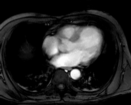
Figure 4.22 Original image of collection mr2
update mr2 as a
set a assign a[0 : 179 , 0:54] + $1/2c
The argument $1 is the arrow image (Figure 4.23) which has to be shipped to the server along with the query. It is an image showing a white arrow on a black background. For more information on the use of $ variables you may want to consult the language binding guides of the rasdaman Documentation Set.

Figure 4.23 Arrow used for updating
Looking up the mr2 collection after executing the update yields the result as shown in Figure 4.24:

Figure 4.24 Updated collection mr2
Note
The replacement expression and the MDD to be updated (i.e., left and right-hand side of the assign clause) in the above example must have the same dimensionality. Updating a (lower-dimensional) section of an MDDs can be achieved through a section operator indicating the “slice” to be modified. The following query appends one line to a fax (which is assumed to be extensible in the second dimension):
update fax as f
set f[ *:* , sdom(f)[1].hi+1 ] assign $1
The example below updates target collection mr2 with data from rgb
(collection that exists already in the database):
update mr2 as a
set a assign b[ 0:150, 50:200 ].red
from rgb as b
4.17.4.1. Partial Updates
Often very large data files need to be inserted in rasdaman, which don’t fit in main memory. One way to insert such a large file is to split it into smaller parts, and then import each part one by one via partial updates, until the initial image is reconstructed in rasdaman.
This is done in two steps: initializing an MDD in a collection, and inserting each part in this MDD.
4.17.4.1.1. Initialization
Updates replace an area in a target MDD object with the data from a source MDD object, so first the target MDD object needs to be initialized in a collection. To initialize an MDD object it’s sufficient to insert an MDD object of size 1 (a single point) to the collection:
insert into Coll
values marray it in [0:0,0:0,...] values 0
Note that the MDD constructed with the marray constructor should match the type of Coll (dimension and base type). If the dimension of the data matches the Coll dimensions (e.g. both are 3D), then inserting some part of the data would work as well. Otherwise, if data is 2D and Coll is 3D for example, it is necessary to initialize an array in the above way.
4.17.4.1.2. Updates
After we have an MDD initialized in the collection, we can continue with updating it with the individual parts using the update statement in rasql.
Refering to the update statement syntax, mddExp can
be any expression that results in an MDD object M, like an marray construct, a
format conversion function, etc. The position where M will be placed in the
target MDD (collAlias) is determined by the spatial domain of M. When
importing data in some format via the decode function, by default the resulting
MDD has an sdom of [0:width,0:height,..], which will place M at [0,0,..]
in the target MDD. In order to place it in a different position, the spatial
domain of M has to be explicitly set with the shift function in the query. For
example:
update Coll as c set c
assign shift(decode($1),[100,100])
The update statement allows one to dynamically expand MDDs (up to the limits of the MDD type if any have been specified), so it’s not necessary to fully materialize an MDD.
When the MDD is first initialized with:
insert into Coll
values marray it in [0:0,0:0,...] values 0
it has a spatial domain of [0:0,0:0,...] and only one point is materialized
in the database. Updating this MDD later on, further expands the spatial domain
if the source array M extends outside the sdom of target array T.
4.17.4.1.3. Example: 3D timeseries
Create a 3D collection first for arrays of type float:
create collection Coll FloatSet3
Initialize an array with a single cell in the collection:
insert into Coll
values marray it in [0:0,0:0,0:0] values 0f
Update array with data at the first time slice:
update Coll as c set c[0,*:*,*:*]
assign decode($1)
Update array with data at the second time slice, but shift spatially to
[10,1]:
update Coll as c set c[1,*:*,*:*]
assign shift( decode($1), [10,1] )
And so on.
4.17.4.1.4. Example: 3D cube of multiple 3D arrays
In this case we build a 3D cube by concatenating multiple smaller 3D cubes along a certain dimension, i.e. build a 3D mosaic.
Create the 3D collection first (suppose it’s for arrays of type float):
create collection Coll FloatSet3
Initialize an array with a single cell in the collection:
insert into Coll
values marray it in [0:0,0:0,0:0] values 0f
Update array with the first cube, which has itself sdom [0:3,0:100,0:100]:
update Coll as c set c[0:3,0:100,0:100]
assign decode($1, "netcdf")
After this Coll has sdom [0:3,0:100,0:100].
Update array with the second cube, which has itself sdom [0:5,0:100,0:100];
note that now we want to place this one on top of the first one with respect to
the first dimension, so its origin must be shifted by 5 so that its sdom will be
in effect [5:10,0:100,0:100]:
update Coll as c set c[5:10,0:100,0:100]
assign shift(decode($1, "netcdf"), [5,0,0])
The sdom of Coll is now [0:10,0:100,0:100].
Update array with the third cube, which has itself sdom [0:2,0:100,0:100];
note that now we want to place this one next to the first two with respect to
the second dimension and a bit higher by 5 pixels, so that its sdom will be in
effect [5:7,100:200,0:100]:
update Coll as c set c[5:7,100:200,0:100]
assign shift(decode($1, "netcdf"), [5,100,0])
The sdom of Coll is now [0:10,100:200,0:100].
4.17.5. Delete
Arrays are deleted from a database collection using the delete statement. The arrays to be removed from a collection can be further characterized in an optional where clause. If the condition is omitted, all elements will be deleted so that the collection will be empty afterwards.
Syntax
delete from collName [ as collAlias ]
[ where booleanExp ]
Example
delete from mr1 as a
where all_cells( a < 30 )
This will delete all “very dark” images of collection mr1 with all pixel
values lower than 30.
4.18. In-Situ File Archive Storage [RE]
While rasdaman establishes efficient access structures in its databases, sometimes service providers do not want to make use of these features due to the extra disk space needed: “I cannot copy my 100 TB into a database.“
The rasdaman in-situ capability provides access to MDD tiles stored in files and directories outside DBMS control. A host of different formats can is understood by rasdaman, and virtually any given archive structure can be accommodated.
Queries on such MDD objects stored in a file system are evaluated “as is”, without importing them into a database first.
4.18.1. Accessing in-situ data
Access to in-situ file data is in no way different from database access: Any select query can be sent to the rasdaman service where the in-situ files have been registered previously. Queries can access both database and in-situ tiles.
4.18.2. Registering in-situ data
Raster data that sits in files get referenced to rasdaman without importing the actual contents, by simply registering these data to the database; only access pertinent metadata are stored in the database.
All files registered in one insert statement must be compatible with the MDD
type indicated.
Any of the formats understood by GDAL can be registered, as well as NetCDF
and GRIB2 data. File formats are detected automatically, therefore the query
does not have any reference to the file format. Files registered within one
insert statement can be of different file format.
The resulting object will have an extent given by the minimal bounding box over all files registered.
Upon registration, the following plausibility checks are performed:
Does the file exist and is it accessible to the rasdaman server?
Is the file type understood by rasdaman?
Does the cell type match the definition given in the
insertstatement?
Syntax
insert into collName referencing ( typeName )
insitu (filePath, covertorType, formatParams, domain),
...,
insitu (filePath, covertorType, formatParams, domain)
where:
identifier collName is the name of the collection that will hold the array,
identifier typeName is the name of the mdd type corresponding to the array,
string filePath is an absolute file path under which the file is accessible by local rasdaman server,
string convertorType is one of “gdal”, “netcdf” or “grib”,
string formatParams any extra format parameters to be passed to the decoder when reading the file,
mintervalExp domain indicates the location where these files are supposed to sit in the newly generated MDD.
Example
In the following we assume greyscale TIFF images g1.tif, g2.tif,
g3.tif, and g4.tif, each of extent 100 x 100 and all sitting in
directory /data/images/*.*. Further, we assume that the resulting object
should be a square of dimensionality 200 x 200, with each of the tiles in a
corner. The following query will generate that:
insert into GreyEx referencing (GreyImage)
insitu("/data/images/g1.tif", "gdal", "", [0:99, 0:99]),
insitu("/data/images/g2.tif", "gdal", "", [100:199, 0:99]),
insitu("/data/images/g3.tif", "gdal", "", [0:99, 100:199]),
insitu("/data/images/g4.tif", "gdal", "", [100:199, 100:199])
The resulting object covers points from the interval [0:199, 0:199].
4.18.3. Updating with in-situ Data
Data sitting in files can be referenced in update statements as well. The referenced data can overlap existing in-situ data. The pixel value is always given by the last file that touched the pixel. Mixing in-situ and imported data in the same array object is currently undefined behaviour.
Syntax
update iteratedColl set updateSpec assign referencing
insitu(filePath, convertorType, formatParams, domain),
...,
insitu(filePath, convertorType, formatParams, domain)
where:
iteratedColl and updateSpec are regular update tokens (see Update section).
string filePath is an absolute file path under which the file is accessible by local rasdaman server
string convertorType is one of “gdal”, “netcdf” or “grib”
string formatParams any extra format parameters to be passed to the decoder when reading the file
mintervalExp domain indicates the region in the file to be referenced.
Example
We assume we want to modify the mdd generated in the insert example such that its middle section pixel values are now read from the file “/data/images/g5.tif” of dimensionality 100*100. The following query will generate that:
update GreyEx set GreyEx[50:149, 50:149] assign referencing
insitu("/data/images/g5.tif", "gdal", "", [0:99, 0:99])
4.18.4. De-Registering in-situ Data
De-registering files associated with an MDD object is done through a rasql
delete statement; this will remove the database MDD object and remove all
knowledge about the previously registered files in the database.
Syntax is identical to the usual delete statement.
If one or more of the files registered are not present any longer at the time of the object deletion this will be ignored gracefully, without aborting query processing.
Note
In a future version, the update statement will be extended to allow
selective de-registration of files registered with an object.
4.18.5. Listing in-situ Data
Listing in-situ data registered with a rasdaman service will be provided in a
forthcoming version, most likely through a describe command.
4.18.6. No Updating or Deleting of in-situ Data
As rasdaman assumes read-only (“guest”) access to the in-situ archive, physical change and deletion of archive files and directories is not possible through rasdaman. See above for de-registering in-situ files.
4.18.7. Errors
Below error messages and situations are explained which can happen during registration, de-registration, and access of in-situ archive data.
“Referenced file not found.”
This error occurs when one or more of the given paths are incorrect. It is always assumed that the paths are absolute. A query which generates this message is:
insert into MyGreyImages referencing (GreyImage)
insitu("/example/not-existing.tif", "gdal", " ", [0:99, 0:49])
if file not-existing.tif is not existing (or not in this directory).
“Referenced path not absolute.”
This error occurs when one or more of the given paths are not absolute. A query which generates this message is:
insert into MyGreyImages referencing (GreyImage)
insitu("my-image.tif", "gdal", " ", [0:99, 0:49])
“MDD type $token unknown.”
This error occurs when the MDD type indicated (reported in $token) does not exist. A query which generates this message is:
insert into MyGreyImages referencing (NonExistentType)
insitu("/example/1.tif", "gdal", " ", [0:99, 0:49])
if no type named NonExistentType is existing in the database.
“MDD and collection types are incompatible.”
This error occurs when the given MDD type is not compatible with the collection type. A query that generates this error is:
insert into MyGreyImages referencing (RGBImage)
insitu("/example/1.tif", "gdal", " ", [0:99, 0:49])
assuming collection MyGreyImages is of type GreySet instead of RGBImage as indicated in the query.
“Query contains overlapping tiles.”
This error occurs when two or more files passed as referencing arguments
have intersecting domains. Such situations are currently only supported in
update queries. A query which generates this error is:
insert into MyGreyImages referencing (GreyImage)
insitu("/example/1.tif", "gdal", " ", [0:50, 0:49])
insitu("/example/2.tif", "gdal", " ", [49:60, 0:49])
These files are indicated to have in common the sector [49:50, 0:49], hence they overlap.
De-registration errors
There are no particular error conditions which pertain to in-situ files as such.
Data access errors
When accessing a file in the course of a select query evaluation, first some plausibility checks are executed to make sure the actual file contents still conforms with rasdaman’s perception, This is necessary as the archive files are not under DBMS control, but can be modified or deleted by archive management software, human administrators, or other entities.
If rasdaman detects an inconsistency during these plausibility checks, query processing aborts with an appropriate error message.
4.19. User-Defined Functions - UDFs [RE]
4.19.1. Overview
Wikipedia teaches, “In SQL databases, User-Defined Functions (UDFs) provide a mechanism for extending the functionality of the database server by adding a function that can be evaluated in SQL statements.” This mechanism is available in rasdaman enterprise, too: Functions whose implementation is provided separately, not implemented in the database engine, can be added at any time and then get invoked as part of expressions in rasql queries. This includes SELECT statements, where the function can be used against data stored in database collections. Conceptually, the function is evaluated once per collection element.
Where the SQL standard distinguishes between scalar and table functions, rasql instead knows scalar and array functions. A scalar function returns only a single value (or NULL), whereas an array function returns a rasdaman array.
UDFs in rasdaman can be used in manifold situations. For ad-hoc functionality extension, a UDF may be defined directly in the database, including the source code implementing the function; this code will be compiled and linked on demand. Alternatively, implementation may be provided externally, as a precompiled shared library. Not only allows this to implement dedicated functionality, but it is a gateway to manifold existing tools which users may want to combine with rasdaman, such as Matlab™, R™, or ScalaPack™ (all trademarks of external tools mentioned here duly respected).
The following subsections detail invocation and management of UDFs.
4.19.2. Invoking a UDF
A UDF behaves like an ordinary rasdaman function and, therefore, can be used in a straightforward way in expressions. The data type of the result is the one specified at the function creation time, so, depending on the result, a UDF expression can return either a scalar or an MDD operand.
The types of both input and output parameter expressions must match with the UDF definition, otherwise an exception is reported.
4.19.2.1. Syntax
namespace . fn ( par1, par2, ..., parn )
where
namespace is an Identifier,
fn is an Identifier,
par1, …, parn are expressions acting as input parameters to f
4.19.2.2. Examples
Assume a package mat for matrix operations, containing an operation
transpose(mddExp) which transposes a matrix. This function can be invoked as
follows:
select encode( mat.transpose( m ), "jpeg")
from MyMatrices as m
4.19.3. Creating a UDF
New functions are defined in rasdaman through the create function statement.
A UDF definition is local to the particular rasdaman database where it is
stored, so it is only known in this context.
4.19.3.1. Syntax
create function namespace . fn
( typeName1 var1, ..., typeNameN varN )
returns typeName
language lang
code
where
namespace is an Identifier that establishes a grouping of functions. Namespace identifiers must be unique within a given database.
fn is an Identifier of the function, used for invoking it in a query. Function names must be unique within a given namespace.
typeName1…, typeNameN are the data types of the function input parameters.
var1, …, varN are parameter names and need to be valid Identifiers.
typeName is the data type of the return value.
lang is the programming language in which the UDF’s body is expressed. Currently supported are:
cpp – this identifies GNU C++ code
python - Python code
code specifies the implementation of the function, and is explained in details in Code body provision.
4.19.3.2. Code body provision
The code implementing the UDF can be provided in two ways: ad-hoc or as an external file. In both variants, the code provided will be compiled and linked into the server engine at runtime.
4.19.3.2.1. In-place code
In the ad-hoc case, the function body is provided as program text enclosed in
begin and end keywords:
begin
code block
end
Note
Python UDFs are not supported with in-place code specification currently, only C++ code is allowed; for specifying Python UDF code see External library.
4.19.3.2.2. External library
Alternatively, the code implementing the function can be provided externally; in
this case, the path leading to the library is specified relative to the
rasdaman UDF directory (/opt/rasdaman/share/rasdaman/udf). Depending on
whether the UDF lang is cpp or python, the external library is
one of:
Compiled shared library:
extern "library.so"
Text file with Python code:
extern "library.py"
The library file must exist and be readable by rasserver. If rasdaman cannot access the specified file it will abort query execution with an exception. For security reasons it is strongly advisable to restrict access to the UDFs so that no unauthorized code modification can be performed.
If the UDF relies on functionality from other libraries which are dynamically
linked, the directories in which the 3rd-party libraries are found may need to
be added to the LD_LIBRARY_PATH environment variable. For example, suppose the
UDF uses functionality from libgdal.so installed in /usr/local/lib; the
env variable may need to be updated as follows if it does not already contain
this path:
export LD_LIBRARY_PATH="/usr/local/lib:$LD_LIBRARY_PATH"
This needs to be done before rasdaman is started, and in the rasdaman user
environment which starts rasdaman. The best way is to put the above line in
/etc/default/rasdaman, and always use sudo service rasdaman start which
automatically loads this configuration file.
Whenever the UDF code is changed, it must be updated in
/opt/rasdaman/share/rasdaman/udf/. Rasdaman watches the UDF directory for
changes and will reload the new UDF. If it appears that the new version has not
been reloaded then it may be necessary to manually restart rasdaman.
4.19.3.3. Parameter types
UDFs can receive and return any rasql atomic type, plus strings, and arrays; the same base type identifiers are used as in rasql:
Data type |
Description |
|---|---|
|
signed 1 byte integer type |
|
unsigned 1 byte integer type |
|
signed 2 bytes integer type |
|
unsigned 2 bytes integer type |
|
signed 4 bytes integer type |
|
unsigned 4 bytes integer type |
|
4 bytes single precision floating point type |
|
8 bytes double precision floating point type |
|
1 bit true/false type |
|
sequence of characters, enclosed in double quotes |
|
multidimensional array |
Note
With array neither cell type nor extent are indicated; detailed
type information is passed dynamically through the C++ API
(r_GMarray class), or the NumPy array object in case of a Python UDF.
4.19.3.4. Examples
In the first example, the function fib() produces Fibonacci numbers. The
source code is provided verbatim as function body (note that no function header
is provided in the code block):
create function math.fib ( long n ) returns long
language cpp
begin
if (n == 0 || n == 1) {
return n;
} else {
return fib(n - 1) + fib(n - 2);
}
end
In the second example, the function avg() belonging to namespace stat receives an array and delivers an unsigned short result. The compiled code is provided by the administrator in UDF subdirectory stat/ as file average.so, and needs to be referenced accordingly:
create function stat.avg( array a ) returns ushort
language cpp
extern "stat/average.so"
If the UDF was implemented in Python, its code might be in file
"stat/average.py" instead. See the next section
for more details on the placement of UDF code, and following sections for
writing C++ and Python external UDF code.
4.19.4. Code location
UDF code is stored in directory /opt/rasdaman/share/rasdaman/udf.
Having many UDFs in the same directory (potentially even with their source code
and related files) may make administration unwieldy. Therefore, the udf/
directory can contain any number of subdirectories, with arbitrary naming and
depth. Note that such subpaths must be indicated correctly in the create
function statement, such as
extern "math/average.so"
For UDF subpaths a convention is used by rasdaman, and it is recommended to follow it for externally provided code, too.
Ad-hoc provided code is compiled by rasdaman into a subdirectory udf/
named after its namespace:
/opt/rasdaman/share/rasdaman/udf/ns/
whereby ns is the identifier of the namespace to which the UDF code belongs.
Note that in such a folder intermediary files may be generated by rasdaman when compiling the UDF. All those files – including those possibly located by the administrator, such as source code, Makefiles, documentation, etc. – are ignored by rasdaman.
4.19.5. Writing C++ UDF Code
Any C++ code can be compiled and linked into rasdaman as a UDF, provided a few conventions are followed:
The external source file must define a function with the same name as the function defined in the UDF from the rasdaman viewpoint.
In a C++ environment, this function must be declared
extern "C"to avoid name mangling.Function input parameters as well as result must match with the corresponding UDF definition.
4.19.5.1. Parameter passing
Parameter passing between the rasdaman engine and UDFs is made as convenient as possible through intelligent transparent conversion:
Numerical values are passed directly. Equivalence between rasql and programming language data type is straightforward as suggested by the type names.
Strings are passed as
char*pointers.Arrays are passed into UDFs and accepted from UDFs as pointers to objects of class
r_GMarray. This class is defined in the rasdaman header filerasodmg/gmarray.hhwhich the UDF code must include (see the raUDFDIR and rasodmg C++ API documentation).Multiple tiles are merged and converted to
r_GMArraybefore rasdaman passes them to a UDF, and arrays returned to rasdaman are converted fromr_GMArrayinto tiles where necessary.In case the array is multi-band, then it is necessary to check how the bands are linearized in the array byte data, which is a
char *pointer. Callingget_band_linearization()on ther_GMarrayobject will returnr_Band_Linearization::PixelInterleavedif full pixels are linearized one after another; otherwise it will returnr_Band_Linearization::ChannelInterleavedwhich would indicate channel-interleaved, where each band in turn is fully linearized starting from the first (index 0) and ending with the last one. In both cases it is recommended to useget_band_iterator(bandId)method on ther_GMarrayobject, which returns anr_Band_Iteratorutility object that allows to iterate through the values of the band, or copy the whole band data into a target buffer of sufficient size. Full details are provided in the documentation of these classes.
4.19.5.2. Error handling
Abnormal return are reported according to regular programming language conventions:
Following standard conventions, numeric data types do not have any reserved value, so they cannot report back error conditions. In other words, rasdaman will accept any value passed back as valid result.
A null pointer passed back (in case of return type string or array) will be interpreted as an error and raise a UDF exception in rasdaman, which will then be reported back to the client which has submitted the overall query.
An exception thrown during UDF execution will be mapped to a rasdaman UDF exception, which will then be reported back to the client which has submitted the overall query.
4.19.5.3. Example 1
Assume the above example function fib() is now implemented as an external
function, to be compiled by the user. The corresponding source code may look as
follows:
extern "C" long fib(long n)
{
if (n == 0 || n == 1)
return n;
else
return fib(n - 1) + fib(n - 2);
}
This source can be compiled into a shared library using
g++ -O3 -fPIC -shared -std=c++11 -Wl,-soname,myfib.so -o myfib.so myfib.cpp \
-lm -ldl -L$(RMANHOME)/lib -lrasodmg -lraslib
The dynamic library file, myfib.so, must be placed in the UDF directory for
use by rasdaman. If it is to become part of namespace math/ it should be
placed into UDF directory math/myfib.so.
4.19.5.4. Example 2
Another example with array input and output is provided below; compiling is
similar to the previous example. This UDF function adds 5 to each value in the
provided array, which is assumed to be of base type char; hence it is similar
to the rasql expression a + 5.
#include "rasodmg/gmarray.hh"
#include <cstdlib>
extern "C" r_GMarray* add5(r_GMarray* a)
{
char* in_array = a->get_array();
size_t array_size = a->get_array_size();
char* res_array = (char*) malloc(array_size);
for (size_t i = 0; i < array_size; ++i)
res_array[i] = in_array[i] + 5;
r_GMarray* ret = new r_GMarray();
ret->set_array(res_array);
ret->set_array_size(array_size);
ret->set_spatial_domain(a->spatial_domain());
ret->set_type_length(sizeof(char));
ret->set_type_structure(a->get_type_structure());
ret->set_type_by_name(a->get_type_name());
return ret;
}
4.19.5.5. Example 3
A final example allows calculating histogram on arrays of type
unsigned short. The code for histogram.cc is shown below:
#include "rasodmg/gmarray.hh"
#include <cstring>
extern "C" r_GMarray* histogram(r_GMarray* m)
{
// number of cells in the GMarray
const auto size = m->spatial_domain().cell_count();
// the array data from the GMarray, casted to the correct type
using InCellType = unsigned short;
auto* inData = reinterpret_cast<InCellType*>(m->get_array());
using OutCellType = unsigned int;
constexpr size_t resultSize = 65536;
auto* outData = new OutCellType[resultSize];
memset(outData, 0, resultSize * sizeof(OutCellType));
// create the histogram
for (r_Bytes i = 0; i < size; ++i) {
outData[inData[i]]++;
}
auto* ret = new r_GMarray();
ret->set_array(reinterpret_cast<char*>(outData));
ret->set_array_size(resultSize * sizeof(OutCellType));
ret->set_spatial_domain(r_Minterval("[0:65535]"));
ret->set_type_length(sizeof(OutCellType));
ret->set_type_structure("marray <ulong, 1>");
ret->set_type_by_name("ULongSet1");
return ret;
}
Below is an example Makefile which compiles the histogram.cc source file, and
installs it into the UDF directory. Place both the Makefile and histogram.cc in
the same directory and invoke make in this directory.
RMANHOME = /opt/rasdaman
UDFDIR = $(RMANHOME)/share/rasdaman/udf
INCDIR = -I. -I$(RMANHOME)/include
OPT = -fPIC -shared -std=c++11 -g -O3
CPP = g++
CFLAGS = -DELPP_NO_DEFAULT_LOG_FILE -DELPP_FEATURE_CRASH_LOG \
-DELPP_STACKTRACE -DELPP_FEATURE_CRASH_LOG \
-DELPP_NO_CHECK_MACROS -DELPP_THREAD_SAFE \
$(DBG) $(OPT) $(INCDIR) -Wl,-soname
LINK = -lm -ldl -L$(RMANHOME)/lib -lrasodmg -lraslib
all: histogram
histogram: histogram.cc
$(CPP) $(CFLAGS),$(UDFDIR)/$@.so -o $(UDFDIR)/$@.so $< $(LINK)
cp $(UDFDIR)/$@.so $(UDFDIR)/lib$@.so
4.19.6. Writing Python UDF Code
Any text file with Python code can be registered in rasdaman as a UDF, provided a few conventions are followed:
The code must define a function with the same name as the function name of the UDF registered in rasdaman.
The Python signature and return value must match the signature of the UDF registered in rasdaman.
4.19.6.1. Parameter passing
Parameter passing between the rasdaman engine and Python UDFs is made as convenient as possible through intelligent transparent conversion; numerical and string values are passed as native Python types, while array values are passed as NumPy arrays in the Python code. There are some specifics to note about array parameter or return values:
An array passed from rasdaman into the Python function may appear transposed, usually if the data was imported in rasdaman from a 2D format such as TIFF, JPEG2000, etc. In this case you would have to transpose it (if the orientation is relevant) with numpy.transpose.
Multiband arrays are passed as a 1-D NumPy array with as many values as there are bands, holding a NumPy array at each index. For example if an RGB array is passed from rasdaman to the Python UDF, then in the Python code each band can be accessed as follows:
red = arg[0] green = arg[1] blue = arg[2]
Complex return types, such as tuples or objects are not supported. Multiple arrays as long as they are of the same shape (spatial domain) can be returned as one multiband numpy array.
4.19.6.2. Error handling
Exceptions thrown by a Python UDF will be captured with all details and logged
in the rasserver log in /opt/rasdaman/log. The relevant rasserver log is
usually the most recent file in the log directory that starts with rasserver,
which can be determined with the command ls -ltr | grep rasserver | tail -n1.
Example output in the rasserver log for an exception raised in a Python UDF:
[ERROR] - 2024-01-25 09:42:51,006, error executing udf,
cause: exception raised in Python UDF code,
traceback (most recent call last):
File "/opt/rasdaman/share/rasdaman/udf/systemtest_tests.py", line 165, in test_raise
raise Exception("invalid argument: " + str(arg))
Exception: invalid argument: 5
4.19.6.3. Logging
Standard output from a Python UDF (stdout and stderr), such as printed with the print function, is captured by rasdaman and logged in the rasserver log. How to find the rasserver log is explained in Error handling.
4.19.6.4. Paths, libraries, versions
If PYTHONPATH is not set for the rasdaman system user then rasdaman
will set it to /opt/rasdaman/share/rasdaman/udf before invoking a Python
UDF. Customizing PYTHONPATH could be done in /etc/default/rasdaman; it
is best to make sure that /opt/rasdaman/share/rasdaman/udf is part of it
in this case.
Generally it is most straightforward to install Python libraries system-wide,
e.g. with apt install, or with sudo pip3 install. Otherwise, it may be
necessary to fiddle with PYTHONPATH.
Rasdaman is compiled against the standard Python versions on the respective OS: Python 3.8 on Ubuntu 20.04 and Python 3.10 on Ubuntu 22.04. Running it with a different Python version may not work well or at all.
Note
On Ubuntu 24.04 or earlier the python UDF functionality requires numpy < 2.
An error “failed to import numpy Python module” when calling a Python UDF
in a query likely indicates a mismatch in the available numpy version,
especially if the latest one was installed with pip. Checking
/opt/rasdaman/log/nohup.out could provide more details.
4.19.6.5. Example 1
In this example we implement mean as a Python UDF. First the UDF code can be
placed in a mean.py file containing:
import numpy as np
def mean(arg):
return np.mean(arg, dtype=np.float64)
The file must be deployed then to
/opt/rasdaman/share/rasdaman/udf/mean.py, and we can register the UDF in rasdaman with
rasql -q 'create function math.mean( array arg )
returns double
language python
extern "mean.py"' --user rasadmin --passwd rasadmin
Now the UDF can be invoked in regular SELECT queries, e.g.
SELECT math.mean(mr2) FROM mr2
Note
Whenever the UDF code is changed, it must be updated in
/opt/rasdaman/share/rasdaman/udf/. If the UDF was deployed in another
directory instead then rasdaman must be restarted in order to load the
new version of the code.
4.19.6.6. Example 2
The following UDF accepts a number of Sentinel-2 and Sentinel-1 bands, a path to a machine learning model as a string, and a question as a string. It runs prediction on the given data and question with the model, and returns an answer as a string.
import numpy as np
import torch
import torchvision.transforms as transforms
import torch.nn.functional as F
import EfFormer
def predict(B02, B03, B04, B08, B05, B06, B07, B11, B12,
B8A, VH, VV, model_path, question_text):
image = get_stacked_image(
[B02, B03, B04, B08],
[B05, B06, B07, B11, B12, B8A],
[VH, VV])
image = process_image(image)
model = torch.jit.load(model_path)
question_tokens = tokenize_question(
question=question_text,
model='bert-base-uncased').unsqueeze(0)
res = model([image, question_tokens])
answer_index = torch.argmax(res, dim=1).item()
answer = get_answer_by_index(answer_index)
return answer
Note
This is incomplete code as the implementation of several function calls have been left out; the main goal of this example is to illustrate that UDFs can be more complex and use machine learning frameworks for example.
The full code could be placed in a file rsvqa_predict.py, which is then
copied to the rasdaman UDF directory; note that in
this case we have additional code in a separate module EfFormer, which also
needs to be copied:
cp rsvqa_predict.py EfFormer.py /opt/rasdaman/share/rasdaman/udf/
Note
Whenever the UDF code is changed, it must be updated in
/opt/rasdaman/share/rasdaman/udf/. If the UDF was deployed in another
directory instead then rasdaman must be restarted in order to load the
new version of the code.
To register the UDF in rasdaman we run the following command:
rasql -q 'create function rsvqa.predict(
array B02, array B03, array B04, array B08,
array B05,array B06,array B07,array B11, array B12, array B8A,
array VH, array VV,
string model_path, string question)
returns string
language python
extern "rsvqa_predict.py"'
The UDF could be invoked in a query as follows
SELECT rsvqa.predict(
B02, B03, B04, B08,
B05, B06, B07, B11, B12, B8A,
VH, VH,
"rsvqa_trained_model.pt",
"What L1 land cover classes are there in the image?"
)
FROM S2_L2A_B02_10m as B02, S2_L2A_B03_10m as B03, S2_L2A_B04_10m as B04,
S2_L2A_B08_10m as B08, S2_L2A_B05_20m as B05, S2_L2A_B06_20m as B06,
S2_L2A_B07_20m as B07, S2_L2A_B11_20m as B11, S2_L2A_B12_20m as B12,
S2_L2A_B8A_20m as B8A, S1_GRDH_IW_DV_VH as VH, S1_GRDH_IW_DV_VV as VV
which may return result such as "water bodies".
4.19.7. Deleting a UDF
A UDF can be deleted from the database if it is not needed anymore. This operation requires the right to modify the database.
Syntax
delete function namespace . fn
Example
delete function math.fib
4.19.8. Listing all UDFs
A list of all UDFs currently registered in the database can be obtained using rasql. The result of this query is a list of 1-D char arrays containing the namespace and the name of the functions in the current instance of the rasdaman database, along with the input parameters and result type of each UDF. Optionally, the output can be formatted as json for easier parsing by tools.
Syntax
list udfs [ in json ]
Example
$ rasql --out string -q "list udfs"
opening database RASBASE at localhost:7001...ok
Executing retrieval query...ok
Query result collection has 1 element(s):
Result object 1: dtm.hillshade (array a, float z, float azimuth) returns array
dtm.slope (array a, float z, float azimuth) returns array
dtm.aspect (array a, float z, float azimuth) returns array
...
rasql done.
$ rasql --out string -q "list udfs in json"
opening database RASBASE at localhost:7001...ok
Executing retrieval query...ok
Query result collection has 1 element(s):
Result object 1: [
{ "namespace": "dtm", "name": "hillshade", "parameters": [{ "name": "a", "type": "array" }, { "name": "z", "type": "float" }, { "name": "azimuth", "type": "float" } ], "returns": "array" }
{ "namespace": "dtm", "name": "slope", "parameters": [{ "name": "a", "type": "array" }, { "name": "z", "type": "float" }, { "name": "azimuth", "type": "float" } ], "returns": "array" }
{ "namespace": "dtm", "name": "aspect", "parameters": [{ "name": "a", "type": "array" }, { "name": "z", "type": "float" }, { "name": "azimuth", "type": "float" } ], "returns": "array" }
...
rasql done.
4.19.9. Retrieving a UDF body
The definition of a UDF, i.e., its function header and body, can be retrieved via rasql as well. The result of this query is the function declaration as provided at creation time.
Syntax
select get function namespace . fn
Example
$ rasql --out string -q "select get function testfunctions.f1"
opening database RASBASE at localhost:7001...ok
Executing retrieval query...ok
Query result collection has 1 element(s):
Result object 1: create function testfunctions.f1
long a, double b, char c
returns double
language cpp
begin
return b;
end
rasql done.
4.20. Transaction Scheduling
Since rasdaman 9.0, database transactions lock arrays on fine-grain level. This prevents clients from changing array areas currently being modified by another client.
4.20.1. Locking
Lock compatibility is as expected: read access involves shared (“S”) locks which are mutually compatible while write access imposes an exclusive lock (“X”) which prohibits any other access:
S |
X |
|
S |
+ |
- |
X |
- |
- |
Shared locks are set by SELECT queries, exclusive ones in INSERT,
UPDATE, and DELETE queries.
Locks are acquired by queries dynamically as needed during a transaction. All locks are held until the end of the transaction, and then released collectively [15].
4.20.2. Lock Granularity
The unit of locking is a tile, as tiles also form the unit of access to persistent storage.
4.20.3. Conflict Behavior
If a transaction attempts to acquire a lock on a tile which has an incompatible lock it will abort with a message similar to the following:
Error: One or more of the target tiles are locked by another
transaction.
Only the query will return with an exception, the rasdaman transaction as such is not affected. It is up to the application program to catch the exception and react properly, depending on the particular intended behaviour.
4.20.4. Lock Federation
Locks are maintained in the PostgreSQL database in which rasdaman stores data. Therefore, all rasserver processes accessing the same RASBASE get synchronized.
4.20.5. Examples
The following two SELECT queries can be run concurrently against the same database:
rasql -q "select mr[0:10,0:10] from mr"
rasql -q "select mr[5:10,5:10] from mr"
The following two UPDATE queries can run concurrently as well, as they address different collections:
rasql -q "update mr set mr[0:10,0:10] \
assign marray x in [0:10,0:10] values 127c" \
--user rasadmin --passwd rasadmin
rasql -q "update mr2 set mr2[0:5,0:5] \
assign marray x in [0:5,0:5] values 65c" \
--user rasadmin --passwd rasadmin
From the following two queries, one will fail (the one which happens to arrive later) because the address the same tile:
rasql -q "update mr set mr[0:10,0:10] assign \
marray x in [0:10,0:10] values 127c" \
--user rasadmin --passwd rasadmin
rasql -q "update mr set mr[0:5,0:5] assign \
marray x in [0:5,0:5] values 65c" \
--user rasadmin --passwd rasadmin
4.20.6. Limitations
Currently, only tiles are locked, not other entities like indexes.
4.21. Linking MDD with Other Data
4.21.1. Purpose of OIDs
Each array instance and each collection in a rasdaman database has a identifier which is unique within a database. In the case of a collection this is the collection name and an object identifier (OID), whereas for an array this is only the OID. OIDs are generated by the system upon creation of an array instance, they do not change over an array’s lifetime, and OIDs of deleted arrays will never be reassigned to other arrays. This way, OIDs form the means to unambiguously identifiy a particular array. OIDs can be used several ways:
In rasql, OIDs of arrays can be retrieved and displayed, and they can be used as selection conditions in the condition part.
OIDs form the means to establish references from objects or tuples residing in other databases systems to rasdaman arrays. Please refer for further information to the language-specific rasdaman Developer’s Guides and the rasdaman External Products Integration Guide available for each database system to which rasdaman interfaces.
Due to the very different referencing mechanisms used in current database technology, there cannot be one single mechanism. Instead, rasdaman employs its own identification scheme which, then, is combined with the target DBMS way of referencing. See Object identifier (OID) Constants of this document as well as the rasdaman External Products Integration Guide for further information.
4.21.2. Collection Names
MDD collections are named. The name is indicated by the user or the application program upon creation of the collection; it must be unique within the given database. The most typical usage forms of collection names are
as a reference in the from clause of a rasql query
their storage in an attribute of a base DBMS object or tuple, thereby establishing a reference (also called foreign key or pointer).
4.21.3. Array Object identifiers
Each MDD array is world-wide uniquely identified by its object identifier (OID). An OID consists of three components:
A string containing the system where the database resides (system name),
A string containing the database (base name), and
A number containing the local object id within the database.
The main purposes of OIDs are
to establish references from the outside world to arrays and
to identify a particular array by indicating one OID or an OID list in the search condition of a query.
4.22. Storage Layout Language
4.22.1. Overview
Tiling
To handle arbitrarily large arrays, rasdaman introduces the concept of tiling them, that is: partitioning a large array into smaller, non-overlapping sub-arrays which act as the unit of storage access during query evaluation. To the query client, tiling remains invisible, hence it constitutes a tuning parameter which allows database designers and administrators to adapt database storage layout to specific query patterns and workloads.
To this end, rasdaman offers a storage layout language for arrays which embeds into the query language and gives users comfortable, yet concise control over important physical tuning parameters. Further, this sub-language wraps several strategies which turn out useful in face of massive spatio-temporal data sets.
Tiling can be categorized into aligned and non-aligned (Figure 4.25).A tiling is aligned if tiles are defined through axis-parallel hyperplanes cutting all through the domain. Aligned tiling is further classified into regular and aligned irregular depending on whether the parallel hyperplanes are equidistant (except possibly for border tiles) or not. The special case of equally sized tile edges in all directions is called cubed.
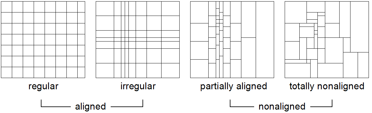
Figure 4.25 Types of tilings
Non-aligned tiling contains tiles whose faces are not aligned with those of their neighbors. This can be partially aligned with still some hyperplanes shared or totally non-aligned with no such sharing at all.
Syntax
We use a BNF variant where optional elements are indicated as
( ... )?
to clearly distinguish them from the “[” and “]” terminals.
Tiling Through API
In the rasdaman C++ API (cf. C++ Guide), this functionality is available through a specific hierarchy of classes.
Introductory Example
The following example illustrates the overall syntax extension which the storage layout sublanguage adds to the insert statement:
insert into MyCollection
values ...
tiling
area of interest [0:20,0:40],[45:80,80:85]
tile size 1000000
4.22.2. General Tiling Parameters
Maximum Tile Size
The optional tile size parameter allows specifying a maximum tile size; irrespective of the algorithm employed to obtain a particular tile shape, its size will never exceed the maximum indicated in this parameter.
Syntax:
tile size t
where t indicates the tile size in bytes.
If nothing is known about the access patterns, tile size allows streamlining array tiling to architectural parameters of the server, such as DMA bandwidth and disk speed.
Tile Configuration
A tile configuration is a list of bounding boxes specified by their extent. No position is indicated, as it is the shape of the box which will be used to define the tiling, according to various strategies.
Syntax:
[ integerLit , ... , integerLit ]
For a d-dimensional MDD, the tile configuration consists of a vector
of d elements where the ith vector specifies the tile
extent in dimension i, for 0lei<d. Each number indicates the
tile extent in cells along the corresponding dimension.
For example, a tile configuration [100, 100, 1000] for a 3-D MDD states
that tiles should have an extent of 100 cells in dimension 0 and 1, and
an extent of 1,000 cells in dimension 2. In image timeseries analysis,
such a stretching tiles along the time axis speeds up temporal analysis.
4.22.3. Regular Tiling
Concept
Regular tiling applies when there is some varying degree of knowledge about the subsetting patterns arriving with queries. We may or may not know the lower corner of the request box, the size of the box, or the shape (i.e., edge size ratio) of the box. For example, map viewing clients typically send several requests of fixed extent per mouse click to maintain a cache of tiles in the browser for faster panning. So the extent of the tile is known – or at least that tiles are quadratic. The absolute location often is not known, unless the client is kind enough to always request areas only in one fixed tile size and with starting points in multiples of the tile edge length.If additionally the configuration follows a uniform probability distribution then a cubed tiling is optimal.
In the storage directive, regular tiling is specified by providing a bounding box list, TileConf, and an optional maximum tile size:
Syntax
tiling regular TileConf ( tile size integerLit )?
Example
This line below dictates, for a 2-D MDD, tiles to be of size 1024 x 1024, except for border tiles (which can be smaller):
tiling regular [ 1024 , 1024 ]
4.22.4. Aligned Tiling
Concept
Generalizing from regular tiling, we may not know a good tile shape for all dimensions, but only some of them. An axis pin { 1, …, d } which never participates in any subsetting box is called a preferred (or preferential) direction of access and denoted as tcp = *. An optimal tile structure in this situation extends to the array bounds in the preferential directions.
Practical use cases include satellite image time series stacks over some region. Grossly simplified, during analysis there are two distinguished access patterns (notwithstanding that others occur sometimes as well): either a time slice is read, corresponding to tc = (*, *, t) for some given time instance t, or a time series is extracted for one particular position (x, y) on the earth surface; this corresponds to tc = ( x, y, *). The aligned tiling algorithm creates tiles as large as possible based on the constraints that (i) tile proportions adhere to tc and (ii) all tiles have the same size. The upper array limits constitute an exception: for filling the remaining gap (which usually occurs) tiles can be smaller and deviate from the configuration sizings. Figure 4.26 illustrates aligned tiling with two examples, for configuration tc = (1, 2) (left) and for tc =(1, 3, 4) (right).
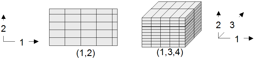
Figure 4.26 Aligned tiling examples
Preferential access is illustrated in Figure 4.27. Left, access is performed along preferential directions 1 and 2, corresponding to configuration tc = (*, *, 1). The tiling tothe right supports configuration tc = (4, 1, *) with preferred axis 3.
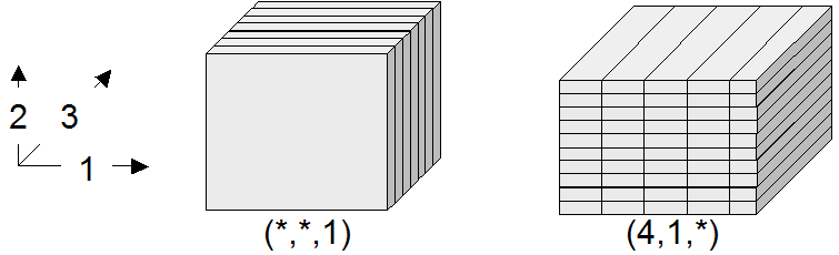
Figure 4.27 Aligned tiling examples with preferential access directions
The aligned tiling construction consists of two steps. First, a concrete tile shape is determined. After that, the extent of all tiles is calculated by iterating over the array’s complete domain. In presence of more than one preferred directions - i.e., with a configuration containing more than one “*” values - axes are prioritized in descending order. This exploits the fact that array linearization is performed in a way that the “outermost loop” is the first dimension and the “innermost loop” the last. Hence, by clustering along higher coordinate axes a better spatial clustering is achieved.
Syntax
tiling aligned TileConf ( tile size IntLit )?
Example
The following clause accommodates map clients fetching quadratic images known to be no more than 512 x 512 x 3 = 786,432 bytes:
tiling aligned [1,1] tile size 786432
Important
Aligned tiling is the default strategy in rasdaman.
4.22.5. Directional Tiling
Concept
Sometimes the application semantics prescribes access in well-known coordinate intervals. In OLAP, such intervals are given by the semantic categories of the measures as defined by the dimension hierarchies, such as product categories which are defined for the exact purpose of accessing them group-wise in queries. Similar effects can occur with spatio-temporal data where, for example, a time axis may suggest access in units of days, weeks, or years. In rasdaman, if bounding boxes are well known then spatial access may be approximated by those; if they are overlapping then this is a case for area-of-interest tiling (see below), if not then directional tiling can be applied.
The tiling corresponding to such a partition is given by its Cartesian product. Figure 4.28 shows such a structure for the 2-D and 3-D case.
To construct it, the partition vectors are used to span the Cartesian product first. Should one of the resulting tiles exceed the size limit, as it happens in the tiles marked with a “*” in Figure 4.28, then a so-called sub-tiling takes place. Sub-tiling applies regular tiling by introducing additional local cutting hyperplanes. As these hyperplanes do not stretch through all tiles the resulting tiling in general is not regular. The resulting tile set guarantees that for answering queries using one of the subsetting patterns in part, or any union of these patterns, only those cells are read which will be delivered in the response. Further, if the area requested is smaller than the tile size limit then only one tile needs to be accessed.

Figure 4.28 Directional tiling
Sometimes axes do not have categories associated. One possible reason is that subsetting is never performed along this axis, for example in an image time series where slicing is done along the time axis while the x/y image planes always are read in total. Similarly, for importing 4-D climate data into a GIS a query might always slice at the lowest atmospheric layer and at the most current time available without additional trimming in the horizontal axes.
We call such axes preferred access directions in the context of a directional tiling; they are identified by empty partitions. To accommodate this intention expressed by the user the sub-tiling strategy changes: no longer is regular tiling applied, which would introduce undesirable cuts along the preferred axis, but rather are subdividing hyperplanes constructed parallel to the preference axis. This allows accommodating the tile size maximum while, at the same time, keeping the number of tiles accessed in preference direction at a minimum.
In Figure 4.29, a 3-D cube is first split by way of directional tiling (left). One tile is larger than the maximum allowed, hence sub-tiling starts (center). It recognizes that axes 0 and 2 are preferred and, hence, splits only along dimension 1. The result (right) is such that subsetting along the preferred axes - i.e., with a trim or slice specification only in dimension 1 - can always be accommodated with a single tile read.
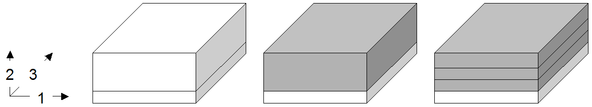
Figure 4.29 Directional tiling of a 3-D cube with one degree of freedom
Syntax
tiling directional splitList
( with subtiling ( tile size integerLit)? )?
where splitList is a list of split vectors (t1,1; …; t1,n1),…,(td,1; …; td,nd). Each split vector consists of an ascendingly ordered list of split points for the tiling algorithm, or an asterisk “*” for a preferred axis. The split vectors are positional, applying to the dimension axes of the array in order of appearance.
Example
The following defines a directional tiling with split vectors (0; 512; 1024) and (0; 15; 200) for axes 0 and 2, respectively, with dimension 1 as a preferred axis:
tiling directional [0,512,1024], [], [0,15,200]
4.22.6. Area of Interest Tiling
Concept
An area of interest is a frequently accessed sub-array of an array object. An area-of-interest pattern, consequently, consists of a set of domains accessed with an access probability significantly higher than that of all other possible patterns. Goal is to achieve a tiling which optimizes access to these preferred patterns; performance of all other patterns is ignored.
These areas of interest do not have to fully cover the array, and the may overlap. The system will establish an optimal disjoint partitioning for the given boxes in a way that the amount of data and the number of tiles accessed for retrieval of any area of interest are minimized. More exactly, it is guaranteed that accessing an area of interest only reads data belonging to this area.
Figure 4.30 gives an intuition of how the algorithm works. Given some area-of-interest set (a), the algorithm first partitions using directional tiling based on the partition boundaries (b). By construction, each of the resulting tiles (c) contains only cells which all share the same areas of interest, or none at all. As this introduces fragmentation, a merge step follows where adjacent partitions overlapping with the same areas of interest are combined. Often there is more than one choice to perform merging; the algorithm is inherently nondeterministic. Rasdaman exploits this degree of freedom and cluster tiles in sequence of dimensions, as this represents the sequentialization pattern on disk and, hence, is the best choice for maintaining spatial clustering on disk (d,e). In a final step, sub-tiling is performed on the partitions as necessary, depending on the tile size limit. In contrast to the directional tiling algorithm, an aligned tiling strategy is pursued here making use of the tile configuration argument, tc. As this does not change anything in our example, the final result (f) is unchanged over (e).
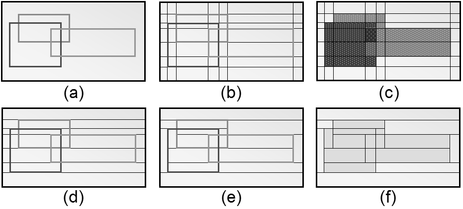
Figure 4.30 Steps in performing area of interest tiling**
Syntax
tiling area of interest tileConf ( tile size integerLit )?
Example
tiling area of interest
[0:20,0:40],[945:980,980:985],[10:1000,10:1000]
4.22.7. Tiling statistic
Concept
Area of interest tiling requires enumeration of a set of clearly delineated areas. Sometimes, however, retrieval does not follow such a focused pattern set, but rather shows some random behavior oscillating around hot spots. This can occur, for example, when using a pointing device in a Web GIS: while many users possibly want to see some “hot” area, coordinates submitted will differ to some extent. We call such a pattern multiple accesses to areas of interest. Area of interest tiling can lead to significant disadvantages in such a situation. If the actual request box is contained in some area of interest then the corresponding tiles will have to be pruned from pixels outside the request box; this requires a selective copying which is significantly slower than a simple memcpy(). More important, however, is a request box going slightly over the boundaries of the area of interest - in this case, an additional tile has to be read from which only a small portion will be actually used. Disastrous, finally, is the output of the area-of-interest tiling, as an immense number of tiny tiles will be generated for all the slight area variations, leading to costly merging during requests.
This motivates a tiling strategy which accounts for statistically blurred access patterns. The statistic tiling algorithm receives a list of access patterns plus border and frequency thresholds. The algorithm condenses this list into a smallish set of patterns by grouping them according to similarity. This process is guarded by the two thresholds. The border threshold determines from what maximum difference on two areas are considered separately. It is measured in number of cells to make it independent from area geometry. The result is a reduced set of areas, each associated with a frequency of occurrence. In a second run, those areas are filtered out which fall below the frequency threshold. Having calculated such representative areas, the algorithm performs an area of interest tiling on these.
This method has the potential of reducing overall access costs provided thresholds are placed wisely. Log analysis tools can provide estimates for guidance. In the storage directive, statistical tiling receives a list of areas plus, optionally, the two thresholds and a tile size limit.
Syntax
tiling statistic tileConf
( tile size integerLit )?
( border threshold integerLit)?
( interest threshold floatLit)?
Example
The following example specifies two areas, a border threshold of 50 and an interest probability threshold of 30%:
tiling statistic [0:20,0:40],[30:50,70:90]
border threshold 50
interest threshold 0.3
4.22.8. Summary: Tiling Guidelines
This section summarizes rules of thumb for a good tiling. However, a thorough evaluation of the query access pattern, either empirically through server log inspection or theoretically by considering application logics, is strongly recommended, as it typically offers a potential for substantial improvements over the standard heuristics.
Nothing is known about access patterns: choose regular tiling with a maximum tile size; on PC-type architectures, tile sizes of about 4-5 MB have yielded good results.
Trim intervals in direction x are n times more frequent than in direction y and z together: choose directional tiling where the ratios are approximately x*n=y*z. Specify a maximum tile size.
Hot spots (i.e., their bounding boxes) are known: choose Area of Interest tiling on these bounding boxes.
4.23. Storage Encoding and Compression [RE]
4.23.1. Specifying Storage Encoding and Compression
4.23.2. Introduction
Storage of arrays in rasdaman is done by partitioning them into tiles, as described already in Storage Layout Language. Each tile is stored as an independent unit. By default, the storage format of tiles is the rasdaman- internal binary format. This is the only format available in rasdaman community; in rasdaman enterprise it is possible to compress tiles or select different storage formats.
The goal of data compression is to transform the data into a more compact but equivalent representation, e.g. using fewer bits to represent frequent symbols and more bits to represent rarely occurring ones. The advantages of using compression are a reduction in storage space and transfer times due to the reduced data volume; the disadvantage is that compression can be demanding on processing power.
4.23.3. Syntax
insert into collName values ...
[ storage encodingFormat [ compression compressionFormat ] ]
where
encodingFormat :
array
| tiff
| hdf
| netcdf
| jpeg
| csv
| png
compressionFormat :
AutoCompression
| ZLib
| SepZLib
| RLE
| SepRLE
| PACKBITS
| TMC
| HaarWavelet
| QHaarWavelet
| DaubechiesWavelet
| Daubechies6Wavelet
| Daubechies8Wavelet
| Daubechies10Wavelet
| Daubechies12Wavelet
| Daubechies14Wavelet
| Daubechies16Wavelet
| Daubechies18Wavelet
| Daubechies20Wavelet
| LeastAsym8Wavelet
| LeastAsym10Wavelet
| LeastAsym12Wavelet
| LeastAsym14Wavelet
| LeastAsym16Wavelet
| LeastAsym18Wavelet
| LeastAsym20Wavelet
| Coiflet6Wavelet
| Coiflet12Wavelet
| Coiflet18Wavelet
| Coiflet24Wavelet
| Coiflet30Wavelet
| Coiflet12Wavelet
By default, encodingFormat is array, i.e. raw byte storage. The
compression subclause is only applicable on array storage encoding format,
e.g. data cannot be encoded in a format like png and then further
compressed.
Note
It is not recommended to use any other format than compressed or uncompressed array. Typically, their decoding overhead is prohibitive with little gain in compression (if at all).
Example
The following query ensures that the inserted array object is stored in tiff format:
insert into mr values $1
storage tiff
We can store a binary mask compressed with RLE for example with the following query:
insert into RiverMasks values $1
storage array compression RLE
4.23.4. Terminology
The compression rate is defined as the average number of bits per cell, so a compression algorithm that achieves a rate of 2 for an 8 bit cell compresses the data to 25% of its raw size. In lossy compression, the rate is no longer limited by the entropy but can be almost arbitrarily small – at the expense of quality, of course. An ideal compression algorithm has minimum rate and minimum loss (= distortion), but unfortunately the minimization of rate and distortion is mutually exclusive. The study of the correlations between rate and distortion is commonly known as rate-distortion theory.
Lossless compression algorithms represent the extreme case of minimum (= 0) distortion at the expense of high rate. In lossy compression, the user can specify a tradeoff between rate and distortion, e.g. achieve very low rates at the expense of quality or vice versa. Therefore an objective measure for the distortion is required in order to evaluate the performance of a lossy compression algorithm. The most commonly used approaches to compare how well a signal \(x\) (consisting of \(n\) samples \(x_1,\ldots,x_n\)) is approximated by a signal \(\hat x\) (also consisting of \(n\) samples \(\hat x_1,\ldots,\hat x_n\)) are the signal-to-noise ratio (\(SNR\)), the peak-signal-to-noise ratio (\(PSNR\)) and the residual (\(Res\)) defined as follows:
\(Snr\) sets the sum of squared sample values (the signal’s energy) in relation to the squared deviation of the approximating signal from the actual one (the error’s energy); \(Psnr\) does the same with the signal’s peak energy. In case there is no error, both \(Snr\) and \(Psnr\) are \(\infty\) and \(Res\) is zero. The differences between these three approaches in plain english:
- SNR
corresponds to the inverse of the average distortion per cell
- PSNR
corresponds to relative amplitude of noise floor
- RES
corresponds to maximum distortion per cell
4.23.5. Compression Engine Architecture
Most modern compression systems have a two-layer architecture consisting of a model layer and a compression layer. The data model in the rasdaman compression engine is that of MDD, i.e. generic multidimensional arrays. By using the semantics of the data stored in MDD format rather than just entropy-coding the MDD’s raster data in some linearization order directly, considerably better compression rates can be achieved. Independently from its actual contents, any MDD has two properties attractive for the model layer:
Base Type: if the base type is structured rather than atomic, it is often more efficient to compress the channels separately rather than the interleaved default. A channel contains all cell values belonging to the same atomic type within a structured type; for instance a colour image (RGB) has three channels, one for each colour.
Spatial neighbourhoods: many objects modelled as MDD have a spatial interpretation (raster images, volume tomograms, spatio-temporal simulations, etc.). Cell values in neighbouring cells are often similar (i.e. correlated) and rarely change rapidly. The way the multidimensional data is linearized within the MDD, spatial neighbourhoods are only visible in one dimension, often leading to suboptimal performance.
It is important to stress the fact that the model layer consists of heuristics and therefore can not guarantee that data compresses better the more heuristics are used. There are MDD over structured base types which compress better if the channels are interleaved, same as there are some MDD where resolving spatial correlations does not improve – or even deteriorate – compression. It is therefore impossible to suggest any compression technique as optimal, since finding the optimum usually requires experimentation. More on this will follow in Hints & Tips.
Compression granularity is also an important issue. Typically a compression algorithm performs better the more data it has to compress; this is because
the relative size of meta data in headers (necessary for correctly decompressing the data) becomes smaller the more data is processed;
many compression techniques are adaptive, i.e. they learn the data properties as they compress the data; that means they have to process a significant amount of data before they are able to compress it efficiently.
On the other hand, the more data is compressed in one unit, the more data needs to be decompressed if any cell within that unit is accessed, so compressing a large MDD as one unit means that accessing any cell within that MDD triggers a decompression of the entire MDD, which will cause the system to grind to a halt. rasdaman already introduced tiles for reduced access granularity, so the natural choice was to make compression operate on tile level as well. Bear in mind that therefore the tile size also represents the compression granularity and keep the tile size reasonably small if access time is more important than storage savings. The default tile size of 32kB is in many cases a good compromise and smaller tiles are discouraged if they are going to be compressed. In some cases considerably larger tiles can also be feasible, however, in particular wavelet compression of MDD with more than two dimensions. Also note that the compression technique can change between tiles of the same MDD, so it is possible to compress some tiles and keep the others uncompressed.
Compression algorithms often require parameters to function efficiently.
For instance ZLib compression allows the user to choose a tradeoff
between compression time and storage savings via a compression level
parameter between 0 (just store) and 9 (best compression at the expense
of speed). The kind and number of parameters can differ considerably
between compression algorithms, therefore a very general system is
needed for the compression parameters. The rasdaman compression engine
supports a dynamic parameter system where the parameters are coded as
strings. A parameter string consists of comma-separated pairs of
keyword=value, where keyword identifies the parameter and
value is the parameter value in string representation. The
interpretation of the value depends on the type of the parameter;
currently three parameter types are supported:
- integers:
32 bit signed integer numbers
- double:
double precision floating point numbers
- strings:
arbitrary-length strings. If the string contains either whitespace characters or commas, it must be enclosed in double quotes, otherwise the double quotes may be omitted.
Some modules also allow vectors of integers or floating point values as
parameters. These have to be entered as strings, and since the values in
these vectors are comma-separated, the strings must be enclosed in
double quotes (e.g. “0,1,2”). Vector types are marked by appending
square brackets [] to the scalar type in the parameter description,
similar to the notation used in languages such as C++.
Note that one parameter string will be used for any compression
operation. This string contains parameters for all modules involved in
the operation and each module extracts those parameters it understands
and ignores all others. An example compression parameter could look like
this (the keywords will be explained in Compression Algorithms):
wavestr=zlib, zlevel=9
4.23.6. Compression Algorithms
The rasdaman compression engine has a two-layer architecture. The compression layer is represented by Compression Streams (see Compression Streams); the various instances of the model layer (see Model Layers) use these compression streams to (de)compress the transformed tile data. In most cases the kind of compression stream to use can be configured via parameters to the model layer.
Compression Streams and Model Layers describe the basic principles of the compression streams and model layers and are recommended reading to understand the compression engine in case you’re unfamiliar with the principles of compression algorithms. Concrete compression formats and their parameters are covered in Model Layer Overview and Parameters.
Model Layer |
\(\longleftrightarrow\) |
Section 4.2 |
Compression Layer |
\(\longleftrightarrow\) |
Section 4.1 |
4.23.6.1. Compression Streams
The compression streams are normally not directly visible to the user, since they are used implicitly by the model layer and not standalone. It is important to describe them, however, to explain the behaviour of the higher layer of the compression engine. There are three types of compression streams available:
- RLE:
(Run Length Encoding). This is a very simple (and hence very fast) compression technique which collapses consecutive identical values and therefore works very well on sparse data, whereas it usually doesn’t achieve any compression at all on dense data.
- ZLib:
This is the well-known standard compression library ZLib, which represents one of the best techniques for lossless compression of arbitrary data. It is a two-layer architecture in itself, with an LZ77 dictionary coder as model layer and Huffmann coding of the resulting dictionary coefficients as compression layer. LZ77 is an adaptive dictionary coding technique which finds repeating patterns in the data stream and replaces matches by a backwards reference into the data already processed and a length count. For example if the most recently processed sequence was
abcbadcbaand the remaining input starts withcbada, thencbadcan be replaced by a backwards reference of -7 and a length count of 4, because the longest matching pattern appeared 7 characters earlier and is 4 characters long. Huffmann coding is entropy-based and represents frequent symbols by fewer bits than infrequent ones, thereby reducing the average number of bits used. ZLib compression usually performs very well and is often either the optimum or reasonably close to it. It has highly asymmetric complexity because of the LZ77 pattern searching phase, however, where compression can take more than 30 times as long as decompression in extreme cases. It is therefore mainly suitable when storage is slow enough that reading less data and decompressing it is faster than reading more uncompressed data.- Arithmetic:
Arithmetic coding (AC) is the state-of-the-art entropy coding technique (superceding Huffmann coding (HC)). It represents a string of input symbols by a number in the unit interval; since the input string can have any length, the number in the unit interval can have very high precision. The main advantage of AC vs. HC is that AC can model any probability distribution exactly and can therefore – at least in theory – get arbitrarily close to the data’s entropy, whereas HC only reaches the entropy if the probabilities of all symbols are (negative) powers of 2. Another advantage is that adaptive AC can be implemented far more efficiently than adaptive HC (the AC in the rasdaman compression engine is also adaptive). Note that AC as a standalone compression technique (i.e. applied to untransformed data) almost always performs worse than ZLib, and frequently worse than RLE as well. AC is only recommended for highly decorrelated data like the output of the wavelet engine’s zerotree coder (for which it is also the default and outperforms all of its rivals).
4.23.6.1.1. Compression Layer Parameters
Currently only the ZLib compression stream supports a parameter for the rate vs. time tradeoff:
Keyword |
Type |
Default |
Description |
|---|---|---|---|
|
integer |
6 |
ZLib compression level between 0 (store only, fast) and 9 (best compression, very slow) |
4.23.6.2. Model Layers
A model layer is responsible for transforming the input data in such a way that the resulting data is no longer correlated. The transformed data is then fed into a compression stream, which should be able to achieve far better compression rates for this decorrelated data. The available model layers fall into three basic categories, ordered in increasing level of complexity:
- None:
no transformation, feed the raw binary tile data with the default cell linearization order into the compression stream.
- Channel separation:
compress each channel separately. This model layer exploits the semantics of structured base types, which means it is equivalent to None if the MDD has an atomic base type.
- Wavelet transformation:
process each channel separately and perform a multiresolution wavelet transformation on the channel data. Wavelet transformations perform spatial decorrelation by applying matching low-pass and high-pass filters to the data along all dimensions, thereby creating bands containing all possible combinations of average (low-pass response) and detail (high-pass response) coefficients for all dimensions (\(2^D\) bands, where \(D\) is the MDD dimension). We define the degree of detail of a band as the number of dimensions in which it holds detail information, so for instance a band with average coefficients in all dimensions has degree of detail 0, whereas a band with average coefficients in one dimension only has degree of detail 1 and so forth. The same procedure is then applied recursively to the band containing the average coefficients in all dimensions until a maximum number of resolution levels has been reached (either limited by the user (parameter
mrlevels) or because the spatial extent of the low-pass response has become too small to allow further filtering). Consider the following examples:- 2D:
(raster image) In the first step, the image with dimensions \(x \times y\) is transformed into four (\(= 2^2\)) bands with sizes \(\frac{x}{2} \times \frac{y}{2}\), where one of those bands is a scaled-down version of the original image (this band contains the average coefficients in both directions) and the other three contain the detail coefficients for three directions (horizontal, vertical, diagonal) which allow reconstructing the original image from the scaled-down version. The same algorithm is then applied recursively to the scaled-down version; a schematic diagram of this procedure can be seen in figure Figure 4.31.

Figure 4.31 This figure shows an example of the band decomposition resulting from multiresolution wavelet transformations. Each band has a name in
{c,d}{c,d}with a resolution level number appended to it (decreasing for coarser levels). The number of the finest level is arbitrary and has no meaning in itself; in the examples it is always chosen such that resolution numbers don’t become negative for simplicity).canddrepresent average (c) and detail (d) information in a given direction, where the first character represents horizontal and the second character vertical direction. The transformation starts with the original image (to the left) at the finest level \(3\) and decomposes this image into bandscc2,cd2,dc2anddd3(in the middle). The same transformations are then applied recursively to bandcc2(to the right) etc. until a coarsest level has been reached.- 3D:
(tomogram) In the first step, the tomogram with dimensions \(x \times y \times z\) is transformed into eight (\(=2^3\)) bands with sizes \(\frac{x}{2} \times \frac{y}{2} \times \frac{z}{2}\), where the band containing the average coefficients in all three dimensions (
ccc2) is again a scaled-down representation of the entire tomogram and the remaining 7 bands contain the detail information in the 7 directions possible for connecting a corner of a cube with the other corners (three along the edges, three diagonals on the faces, one diagonal through the cube, resulting in bandsccd2,cdc2,cdd2,dcc2,dcd2,ddc2andddd2). The same procedure is then applied recursively to the band containing only average coefficients along all directions.
Provided the data matches the wavelet filter, most of the detail coefficients will be very small and can be set to zero without noticeably affecting the quality of the reconstructed data (using the inverse wavelet transformation). That means that the detail coefficients are sparse and therefore highly compressible. Depending on whether the coefficients are stored with sufficient precision to allow reconstructing the original data exactly, wavelet compression techniques fall into two subclasses for lossless and lossy operation.
Any of these base categories can furthermore be combined with so-called predictors (see Predictor Overview and Parameters), an additional model layer which expresses a cell’s value as the difference of the actual cell value from an approximated value (using neighbouring cells to calculate the approximated value). Depending on where the neighbouring cells used for the prediction are located, predictors fall into two categories:
- interchannel:
the neighbouring cells are in the other channels at the same position, so for instance in an RGB image the approximated value of the cell at position \(p\) in channel \(c\) could be calculated using the cells at position \(p\) in any set of channels \(\{c' : c' \ne c\}\). The rasdaman compression engine only allows one predicting channel \(c'\) for each predicted channel \(c\), however;
- intrachannel:
the neighbouring cells are in the spatial neighbourhood of the same channel, so for instance the approximated value of the cell at position \(p\) in channel \(c\) could be calculated using the cells at positions \(p + z\) in channel \(c\) (where \(z\) is an offset vector or a set thereof).
Note
Wavelet transformations can not be combined with intrachannel predictors because both do spatial decorrelation and would therefore compromise each other’s performance. Apart from this exception, the basic model layers and predictors are completely orthogonal concepts and can be combined arbitrarily.
4.23.6.2.1. Model Layer Overview and Parameters
In this section, the various data formats and their parameters will be
explained. The names of the data formats will be given as listed in the
rView Preferences window; programmers using the formats must include
the raslib/mddtypes.hh header file and prefix this name by r_ (r
+ underscore). Note that a tile’s data format can change after updates,
so creating an MDD where the tiles have a given data format \(X\)
does not mean tiles will be stored in data format \(X\) on
subsequent updates; the data format of new/modified tiles is the data
format selected for the current update operation, not the format of the
database tiles being updated.
All model layers allow enabling predictors using the following parameters (note: intrachannel prediction is not available for wavelets; predictors are described in more detail in Predictor Overview and Parameters):
Keyword |
Type |
Default |
Description |
|---|---|---|---|
|
string |
Name of
interchannel
predictor (off
by default).
Possible names
are |
|
|
string |
Name of
intrachannel
predictor (off
by default; not
available for
wavelets).
Possible names
are
|
The following model layers are currently available:
- No Compression:
(data format
Array) This is the default data format for tiles and disables compression entirely for these tiles. For local operation with high bandwidth this format usually performs best because there is no CPU overhead for (de)compression. For low bandwidths, e.g. over the internet, performance can be very bad, however, because in this case less time will be needed for (de)compression than for transferring the additional data volume caused by lack of compression.- No Transformation:
(data formats
RLE,ZLib) In this format, the binary tile data is written directly into a compression stream without any previous transformation. The binary tile data is in default linearization order which hides spatial neighbourhoods in all dimensions but the last one (as a consequence of the default linearization order), and interleaves cell values. Consequently, there is no transformation overhead to speak of and the (de)compression speed of tiles in this format depends entirely on the speed of the underlying compression stream.RLEworks very well for sparse data (i.e. many consecutive identical values), where it is typically within 5%–10% of the compression rate ofZLib, but at a much higher speed. This makesRLEattractive for transfer compression (even over 10Mbit/s ethernet), in particular because it has only slightly asymmetric complexity for compression and decompression. On the downside,RLEachieves no compression at all for dense data.ZLibis one of the most efficient standards for lossless compression and achieves very good compression rates (within the entropy limits) for most data types. It has highly asymmetric complexity for compression and decompression, however, which makes it unattractive for transfer compression where the compression overhead can easily exceed the savings in transfer time. Decompression is very fast, on the other hand, so in case data is read more often than written, it is very likely that overall system performance will improve if the tiles are stored inZLibformat in the database.- Channel separation:
(data formats
SepRLE,SepZLib) In this format, the channels are compressed separately, but no spatial data neighbourhoods are exploited. Thus channel separation can often lead to better compression rates (compared to No Transformation) for MDD over structured base types such as RGB images; for MDD over atomic base types, these data formats are equivalent to the No Transformation ones. The underlying compression streams are the same as in the No Transformation case and the same comments apply. There is a small additional overhead caused by the channel separation, which is noticeably mostly in case of RLE compression (due to RLE’s speed), however.- Wavelet transformations:
wavelet transformations are based on filters with specifiv lengths and shape properties. The shape allows grouping the filters into families (such as Daubechies or Coiflet, see below) and the longer a filter, the better it usually is at analysing smooth data (i.e. less information is contained in the detail coefficients, making the detail bands sparser than shorter filters).
As far as processing complexity is concerned, wavelet transformations are very demanding and not recommended for transfer compression unless the bandwidth is particularily low. This is true in particular for lossy wavelets with zerotree quantization.
The order in which the wavelet bands (see figure Figure 4.31) are processed when using lossless wavelets or bandwise homogeneous quantization is determined by a band iterator which groups detail bands into equivalence groups (identifying each group with an integer number) and iterates over these equivalence groups in sequence. This system is used to process bands consecutively which are expected to share similar properties, in order to optimize the performance of adaptive compression streams. Note that the type of the band iterator does usually not have a large influence on the compression of lossless wavelets but mostly on lossy wavelets because in this case it also groups bands into statistical units. For lossy wavelets, the use of bandwise homogeneous quantization is strongly discouraged, however, since the default zerotree quantization achieves much better compression rates and is also considerably easier to use. For all band iterators, the total average band is always in its own equivalence group 0, which is the first one processed. The following band iterator types are available:
- isolevel:
bands on the same resolution level form an equivalence group. Iteration starts on the coarsest level and proceeds to the finer levels;
- leveldet:
bands on the same resolution level and with the same degree of detail form an equivalence group. Iteration starts on the coarsest level with degree of detail 1 and increments first degree of detail until it has reached its maximum \(D\), then resets the degree of detail to 1 and proceeds to the next finer level;
- isodetail:
bands with the same degree of detail form an equivalence group. Iteration starts with degree of detail 1 and iterates over all bands on all levels with this degree of detail, starting from the coarsest level. Then the degree of detail is incremented and the algorithm continues likewise.
All wavelet compression algorithms understand the following parameters:
Keyword
Type
Default
Description
wavestrstring
ZLib/ArithA colon-separated list of compression stream(s) to use (e.g.
RLE:Ari thwould first RLE-code the data and send the output to an arithmetic coder. Possible stream names areRLE,ZLibandArith(case is irrelevant). The default is a ZLib stream for everything but zerotree coding (lossy wavelets) and an adaptive arithmetic coder for zerotree codingmrlevelsint
0
Maximum number of multiresolution levels to use for the wavelet transformation (compare with figure [FigureWaveExa mple]) . 0 means use the maximum number possible. Sometimes the numerical stability can be improved by reducing the number of resolution levels, in particular for low rates
banditerstring
leveldetPossible values are
isolevel(group by resolution level),leveldet(group by resolution level and degree of detail) andisodetail(group by degree of detail). The band iterator is ignored if zerotree coding is usedThere are lossless and lossy wavelet classes available. Because wavelets perform by far the best if loss is acceptable, there is a strong bias on lossy compression in the wavelet classes.
Lossless wavelets (data format
HaarWavelet). There is currently only one lossless wavelet type, namely the Haar wavelet with a filter length of 2. Note that this filter is lossless for integer base types only, whereas loss in the general area of the machine precision can’t be avoided for floating point types. The performance of this filter depends largely on the MDD kind; in many casesZLiborSepZLibwith an appropriate intrachannel predictor perform better in both compression rate and time taken.Lossy wavelets (data formats
QHaarWavelet(length 2),DaubechiesWavelet(length 4),DaubechiesNWavelet(\(N \in \lbrack 6, 20 \rbrack, N mod 2 = 0\)),LeastAsymNWavelet(\(N \in \lbrack 8, 20 \rbrack, N mod 2 = 0\)),CoifletNWavelet(\(N \in \lbrack 6, 30 \rbrack, N mod 6 = 0\))). In lossy wavelet compression, many of the orthogonal wavelet filters published in the standard literature are supported. The filters used belong to three basic families, the Daubechies family, the LeastAsymmetric family and the Coiflet family; numbers within the filter name describe the length of the filter, soCoiflet30Waveletis a wavelet filter of the Coiflet family with a filter length of 30. As already mentioned above, longer filters are usually better at compressing smooth signals, at least for low-to-moderate rates (shorter filters tend to perform better on all kinds of MDD for high rates).Generic wavelet filters are floating point numbers, so applying such a filter to an MDD channel results in a floating point array of wavelet coefficients (i.e. a data expansion) which has to be quantized efficiently to achieve compression. There are two approaches possible here, bandwise homogeneous quantization (the older, simpler method) and generalized zerotree coding. In bandwise homogeneous quantization, the band iterator partitions the bands into equivalence groups and the quantizer assigns a constant number of bits per coefficient to each band equivalence group; the band data thus quantized is then fed into the compression stream. Generalized zerotree coding successively refines the approximation of the wavelet coefficients and achieves substantial compression by exploiting correlations between coefficients on neighbouring resolution levels. Zerotree coding almost always performs substantially better than bandwise homogeneous quantization in terms of compression rate and offers very simple control over the approximation quality, but it is also considerably more demanding on CPU power. Zerotree coding is the default quantization technique for lossy wavelets and using bandwise homogeneous quantization is discouraged.
All lossy wavelets accept the following parameters:
Keyword
Type
Default
Description
wqtypestring
zerotreeThe quantization technique, can be
zerotreeorperbandenhancelvinteger
0
Enlarge the wavelet coefficients at the boundary of each band on the \(n\) finest levels (where \(n\) is the value of this parameter) before quantization (and reverse this operation after dequantization) to reduce boundary artifacts, in particular for low rates. This ensures that the boundary coefficients are encoded with more precision than the other coefficients.
Most parameters of the compression engine deal with the quantization of wavelet coefficients for lossy wavelet compression. The following terms are important for bandwise homogeneous quantization:
relative number of bits means relative to the size of the base type of the original channel, i.e. quantizing an 8 bit channel with relative number of bits 0.5 means 4 bits per coefficient;
the band group number is determined by the band iterator (see the paragraph about band iterators above).
The following compression parameters are available for bandwise homogeneous quantization:
Keyword
Type
Default
Description
qrtypestring
constSet the relative number of bits to use per band group as a function. Possible values are:
const(constant number of bits),linear(linearily decreasing with increasing group number),expnt(exponentially decreasing with increasing group number),gauss(squared-expone ntially decreasing with group number),custom(is implicitly activated by therelqbitsparameter and can’t be selected directly)qntypestring
linearSet the quantization technique, which can be
linear(same resolution everywhere) andexpnt(higher resolution around 0). If the data is highly concentrated around 0, the exponential quantizer can reduce the average quantization errorbitscaledouble
1
Scale factor for the curves defined by the
qrtypeparameter (except forcustom)relqbitsdouble[]
Vector of doubles which specifies the relative number of bits for each band group, implicitly selects qrtype=custom The interpretation depends on the band iterator chosen
cutoffdouble
1
The number of the cutoff band group relative to the total number of band groups, starting from which band groups should be ignored entirely (i.e. quantized to 0)
nullzonedouble
0
Quantize all coefficients with an absolute value smaller than
nullzoneto 0As can be seen from these parameters, configuring bandwise homogeneous quantization is rather complicated and also dependent on external components like the band iterator. Zerotree coding is much easier to configure and offers much better control over the quantization fidelity.
Remember the distortion measures defined in Terminology which compared the original signal with the approximated signal. Similar to this, distortion measures \(Snr_w\), \(Psnr_w\) and \(Res_w\) can be defined which compare the original wavelet coefficients with the quantized (distorted) coefficients. Zerotree coding uses one of these three alternative distortion measures (selected by the user) as a termination criterion deciding when the coefficients have been encoded with sufficient precision and allows meeting that distortion threshold very closely. It is important to understand the difference between the distortion measures with and without the \(w\) index: with the \(w\) index they describe the distortion of the wavelet coefficients, without the \(w\) index they describe the distortion of the signal reconstructed from these coefficients. Both are loosely related, but the errors of the wavelet coefficients can be amplified in the reconstructed signal. Most importantly it is not possible to predict the distortion of the reconstructed signal from the distortion of the wavelet coefficients precisely enough to be practicable; you have to run tests to see how these two distortions are correlated for your data and the wavelet filter you intend to use.
The following parameters apply to zerotree quantization (where \(Snr_w\) coding is the default and \(Snr_w\), \(Psnr_w\) and \(Res_w\) coding are mutually exclusive):
Keyword
Type
Default
Description
zttypestring
band1Set the zerotree coding algorithm. Possible values are
band1(one-pass coding),band2(two-pass coding with dominant and subordinate pass, corresponds to original zerotree coder)snrdouble[]
\(10^4\)
Use \(SNR_w\) coding, terminating when the \(SNR_w\) of the wavelet coefficients is at least as large as this threshold value. The parameter is a vector of doubles because it is possible to specify different \(SNR_w\) values for each channel
psnrdouble[]
0
Use \(PSNR_w\) coding, otherwise like \(SNR_w\)
residuumdouble[]
0
Use \(RES_w\) coding, terminate when no approximated coefficient differs from its actual value by more than \(RES_w\)
The difference between one-pass and two-pass coding is beyond the scope of this manual. Neither approach performs universally better than the other and neither is dramatically worse than the other in specific cases. The ideal coder must be determined experimentally for the user’s data and wavelet filter.
4.23.6.2.2. Predictor Overview and Parameters
Predictors are classified into intrachannel predictors and interchannel predictors, depending on whether they use cell values in spatially neighbouring cells or in neighbouring channels for prediction. Both types can be added to any of the model layers described above, with the exception of wavelet compression which does not support intrachannel prediction. Prediction first calculates an approximative value for a cell using neighbouring cells (neighbouring in either sense listed above) and then expresses this cell value as the difference (delta) of the actual value from the approximated value. The predictor processes the cells in such an order that the approximated values need not be stored explicitly but can be calculated by the inverse predictor from the cell values it already decoded, thus only the deltas have to be stored. If the predictor model matches the data well, most deltas will be concentrated around 0 and compress better than the untransformed values.
4.23.6.2.3. Interchannel Predictors:
Interchannel predictors approximate the value of a cell at position \(p\) in channel \(c\) by the value of a cell at the same position, but in a different channel \(c_p\). The values of channel \(c\) are then replaced by the difference to the predicted values, resulting in a delta channel. Provided the channels are correlated (as for instance often happens in colour images where brightness influences all three base colours), the value range of the delta channel will be smaller than that of the original channel, thereby allowing more efficient compression. All interchannel predictors require information about the \(c\!:\!c_p\) mappings, which is done by the following parameter:
Keyword |
Type |
Default |
Description |
|---|---|---|---|
|
string |
Comma-separated
list of channel
mappings
\(c\!:\!c_
p\)
where \(c\)
is the number
of the channel
being predicted
and \(c_p\)
is the
predicting
channel
(channel
numbers start
from 0). Take
care that no
cyclic
dependencies
are allowed
(such as
|
There are currently two interchannel predictors available:
- delta:
this predictor just uses the values of channel \(c_p\) directly as approximative values, for channel \(c\) which is recommended if channels are correlated and cover a similar value range, as e.g. often found in RGB images.
- scaledelta:
this predictor first transforms the values of channel \(c_p\) such that they cover the same value range as those of channel \(c\) and uses the resulting values for prediction. This approach is recommended if the channels are correlated, but cover different value ranges (such as temperature and pressure in simulation data).
4.23.6.2.4. Intrachannel Predictors:
Intrachannel predictors approximate the value of a cell at position \(p\) in channel \(c\) by the values of cells at positions \(\{p + z_i\}\) where \(z_i\) are offset vectors describing the relative positions of all cells used for prediction (the predictor context). The available intrachannel predictors all calculate the approximated value as \(\frac{\sum_i w_i v(p + z_i)}{\sum_i w_i}\), where \(v(x)\) is the cell value at position \(x\) and \(w_i\) is the weight for the cell at offset \(z_i\) in the predictor context. The predicted cell’s value is then replaced by the difference to the approximated value and the iteration continues. As can be seen, intrachannel predictors write the deltas to the same channel they read the approximating values from, therefore care had to be taken to process cells in such an order that the inverse predictor can reconstruct the original data.
Currently there are three intrachannel predictors available:
- hyperplane:
this predictor approximates a cell value by the value of the cell at offset \((-\delta_{0,k},\ldots,-\delta_{D-1,k})\), where \(D\) is the number of dimensions, \(k\) is the user-defined prediction direction (\(0 \le k < D\)) and \(\delta_{i,j}\) is the delta function which is \(1\) for \(i = j\) and \(0\) otherwise. For example in the 3D case, the predictor context can be the cell at offset \((-1,0,0)\) (\(k=0\)), the cell at offset \((0,-1,0)\) (\(k=1\)) or the cell at offset \((0,0,-1)\) (\(k=2\)). Thus neighbouring rows or columns will be used for prediction in a 2D MDD, neighbouring planes orthogonal to one axis in a 3D MDD and so forth. The value of \(k\) can be configured with the
hypernormparameter described below.- neighbours:
this predictor uses a subset of the cells whose position differs from that of the predicted cell by at most 1 in all dimensions for prediction. The set of all these cells has to be reduced to allow the inverse predictor to reconstruct the original data; for instance in the 2D case, the predictor context consists of the cells at offsets \((-1,-1)\), \((-1,0)\), \((-1,1)\) and \((0,-1)\) (an L-shaped set of cells). The approximating value is then calculated by using identical weights for all cells.
- weighted:
this predictor uses the same predictor context, but different weights for diagonal cells. Each weight is initialized to 1 and then multiplied by a factor \(f\) for each dimension in which the position of the predicting cell differs from that of the one being predicted. For example in 2D, the cells at offsets \((-1,-1)\) and \((-1,1)\) would have weight \(f^2\) and the cells at offsets \((-1,0)\) and \((0,-1)\) would have weight \(f\). This technique allows reducing or enhancing the influence of diagonal cells on the approximated value, depending on the value of \(f\) which can be configured with the
predweightparameter described below.
Some of these intrachannel predictors also allow configuration via compression parameters. The following parameters are currently available:
Keyword |
Type |
Default |
Description |
|---|---|---|---|
|
string |
|
Comma-separated
list of channel
numbers to use
the predictor
on (starting
from 0). The
exclamation
mark negates
this list, so
the default
value |
|
integer |
0 |
Hyperplane prediction only: the number of the dimension orthogonal to the prediction hyperplane, i.e. the prediction direction (starting from 0) |
|
double |
0.5 |
Weighted neighbours prediction only: the amount a neighbouring cell’s weight is scaled by for every dimension where its coordinate differs from that of the predicted cell. |
4.23.6.2.5. Other Parameters
In contrast to the compression parameters described so far, which are applicable to both storage and transfer compression, the following parameter is only relevant for transfer compression.
Keyword |
Type |
Default |
Description |
|---|---|---|---|
|
integer |
0 |
If
|
Without this parameter it would be impossible to transfer an MDD to the client uncompressed that was stored compressed in the database. This problem may arise if there is a high bandwidth connection between server and client and the client has too little processing power for transparent decompression (or no decompression capabilities at all, such as the RasJ Java binding).
4.23.7. Examples
In the following examples, format: fmt means you have to use the
data format fmt, params: str means you have to use the
parameter string str and defaults: dstr means that
additionally the default parameters described by dstr will be used
implicitly. In rView, you can specify both by opening the preferences
window and scrolling to the bottom, where configurations for storage and
transfer compression can be found. If you use the C++ binding directly,
you have to call your r_Database object’s set_transfer_format()
or set_storage_format() method. For test purposes we recommend
storing the test data uncompressed in the database and experimenting by
changing transfer compression settings and loading the data to the
client via lookups or queries. Once you’ve found satisfying data formats
and/or parameters, you can copy the transfer compression configuration
to the storage compression configuration and then store your test data
in the database with these settings.
Compress using
RLE:format:
RLECompress using
ZLibwith the default compression level:format:
ZLibdefaults:
zlevel=6Compress using
ZLibwith a user-defined compression level (7):format:
ZLibparams:
zlevel=7Compress using
RLEand thedeltainterchannel predictor, using channel 1 to predict channels 0 and 2:format:
RLEparams:
predinter=delta, intermap="0:1,2:1"Compress using
ZLiband thehyperplaneintrachannel predictor with the default prediction direction:format:
ZLibparams:
predintra=hyperplanedefaults:
zlevel=6, hypernorm=0Compress using
ZLibwith thedeltainterchannel predictor predicting channel 0 by channel 1, and thehyperplaneintrachannel predictor using the second dimension as user-defined prediction direction:format:
ZLibparams:
predinter=delta, intermap="0:1" , predintra=hyperplane, hypernorm =1defaults:
zlevel=6Compress using the lossless Haar wavelet with the default compression stream and band iterator:
format:
HaarWaveletdefaults:
wavestr=zlib, zlevel=9, banditer=leveldet, mrlevels=0Compress using the lossless Haar wavelet with an RLE compression stream:
format:
HaarWaveletparams:
wavestr=rledefaults:
banditer=leveldet, mrlevels=0Compress using the lossless Haar wavelet with a compression stream bank of ZLib followed by arithmetic coding and the
deltainterchannel predictor using channel 1 to predict channels 0 and 2:format:
HaarWaveletparams:
wavestr="zlib:arith", predinter =delta, intermap="0:1,2:1", bandi ter=leveldet, mrlevels=0Compress using the lossy Haar wavelet with the default quantization, the default zerotree type, the default termination criterion, an \(Snr_w\) of 100 for all channels and the default compression stream (arithmetic coder):
format:
QHaarWaveletparams:
snr=100defaults:
wqtype=zerotree, zttype=band1, wavestr=arith, enhancelv=0, mrlev els=0Compress using the lossy Haar wavelet with two-pass zerotree quantization, \(Psnr_w\) coding with a \(Psnr_w\) of 300 for all channels and the default compression stream:
format:
QHaarWaveletparams:
zttype=band2, psnr=300defaults:
wqtype=zerotree, wavestr=arith, enhancelv=0, mrlevels=0Compress using the lossy 4-tap Daubechies wavelet with the default quantization, the default zerotree type, \(Res\) coding with a maximum residual per cell of 0.1 for the first channel, 0.2 for the second channel and 0.3 for all other channels, and the default compression stream:
format:
DaubechiesWaveletparams:
res="0.1,0.2,0.3"defaults:
wqtype=zerotree, zttype=band1, wavestr=arith, enhancelv=0, mrlev els=0Compress using the lossy 6-tap Coiflet wavelet with bandwise homogeneous quantization with the default quantizer, quantization, band iterator and compression stream:
format:
Coiflet6Waveletparams:
wqtype=perbanddefaults:
qrtype=const, qntype=linear, bi tscale=1, cutoff=1, nullzone=0, b anditer=leveldet, wavestr=zlib, e nhancelv=0, mrlevels=0Compress using the lossy 20-tap Daubechies wavelet with 3 multiresolution levels, bandwise homogeneous quantization with customized quantizer, exponential quantization,
isolevelband iterator and RLE compression stream:format:
Daubechies20Waveletparams:
mrlevels=3, wqtype=perband, rel qbits="1, 0.75, 0.5, 0.25", qntyp e=expnt, banditer=isolevel, waves tr=rledefaults:
qrtype=custom, cutoff=1, nullzo ne=0, enhancelv=0
4.23.8. Hints & Tips
This section was written to provide some rules of thumb to reduce the vast amount of combinations possible with the compression engine to a manageable size depending on the kind of MDD that should be compressed. While it is not possible to a priori state an optimal compression technique for a given MDD, it is often possible to rule out several approaches entirely, which reduces the complexity of finding the optimal one considerably. Note, however, that all suggestions following below are heuristics and it is perfectly possible that they result in suboptimal compression for some MDD.
4.23.8.1. Hints for Lossless Compression
Lossless compression is easier to handle than lossy compression because it doesn’t require the user to specify a rate-distortion tradeoff since the distortion is always 0. Consequently there are only few model layers with a small set of parameters available for this type of compression; but combined with predictors, there are many combinations possible all the same.
Use
SepZLiborSepRLErather thanZLiborRLEfor multichannel data. UsingSepZLiborSepRLEon data consisting of one channel only introduces some CPU overhead and basically identical compression rate (except for additional header meta data).The lossless Haar wavelet has in many cases inferior compression rate compared to
ZLibwith a suitable intrachannel predictor. Its use is therefore discouraged.ZLibis almost always the best compression stream for the lossless Haar wavelet.RLEandSepRLEonly achieve compression on sparse data (many neighbouring cells have identical values, typically 0), on dense data they only introduce CPU overhead for compression but fail to reduce the data.On sparse data, the compression rates achievable with
RLEandSepRLEare typically not far removed from those ofZLibandSepZLib, but RLE compression is far less demanding on the CPU and is therefore advantageous if speed is critical.
4.23.8.2. Hints for Lossy Compression
Lossy compression – which here always implies wavelet compression – represents the biggest and most complex part of the rasdaman compression engine. It is also the most complex to configure because it requires the user to set a tradeoff between rate and distortion via encoding quality parameters. While in many cases “lossy” algorithms can be made lossless by setting the encoding quality parameters to sufficiently high values, this is discouraged because the compression rate is almost always clearly inferior to that achieved by dedicated lossless compression techniques.
Never use lossy compression for data transfer from client to server unless you fully understand the implications, not even if you want to store the data compressed in this format in the server. The server may have to retile and recompress the data, thereby performing another lossy compression of your data.
Always use zerotree quantization with the adaptive arithmetic coder as compression stream (these are the defaults anyway). Bandwise homogeneous quantization is faster, but its compression rates are way inferior to those of zerotree quantization, in particular for low rates.
Quality parameters: \(Snr_w\) coding models the inverse average distortion per cell, \(Psnr_w\) coding models the relative amplitude of the noise floor and \(Res_w\) coding models the maximum distortion per cell. So for instance if you want to make sure that no coefficient is encoded with a higher error than a given threshold value, use \(Res_w\) coding.
The quality parameters concern the quantization of the wavelet coefficients and do not directly represent the distortion in the reconstructed data. Tests showed that typically the maximum error of the reconstructed data is by a factor of 2–3 larger than the maximum error of the wavelet coefficients, depending on the number of dimensions and the number of resolution levels.
One-pass zerotree coding is often more efficient for predominantly dense data, whereas two-pass zerotree coding is more efficient for predominantly sparse data. For low rates, the differences between the two techniques are minute, however, and usually are quite small for high rates as well.
Long filters (in excess of 8 taps) are usually only advantageous for smooth data and low quality. Many tests showed that for lossless or near lossless compression the Haar wavelet (2 taps) performed best. The Haar wavelet also has the fewest boundary artifacts.
The biggest difference between filters in most tests was their length, not their family. so do not expect big differences in the performance of two 6-tap filters from different families.
4.23.8.3. Hints for Predictors
Predictors can often improve the compression rate considerably, but it is impossible to make definite statements about whether a specific predictor will achieve a positive effect for a given MDD; this must be determined by experiment.
- interchannel predictors
(Interchannel Predictors:) are probably most attractive for multichannel raster images (RGB in the most popular case) where the channels often have substantial correlation (such as grey areas in RGB images). Use the
deltapredictor in these cases.- intrachannel predictors
(Intrachannel Predictors:) come in two complexities, low (
hyperplane) and high (neighbours,weighted). While the predictor overhead per cell is constant forhyperplane, it increases with the number of dimensions forneighboursandweighted. Oftenhyperplaneworks better than its more complex counterparts, in particular if the data has a major correlation direction andhypernormis set to that direction.
4.23.9. Errors
Below error messages and situations are explained which can happen when explicitly specifying storage format encoding or compression.
“Error in compression engine.”
This error indicates a general error with the selected compression scheme. The server logs can be further indicative about the specific error condition.
“Base type not supported by conversion/compression module.”
The selected format encoding or compression scheme does not support encoding or compressing data of this type.
“Invalid storage format specified, compression only applicable on array format.”
This error will occur when compression is attempted on encoded data, e.g:
insert into RiverMasks values $1
storage png compression ZLib
“Unsupported compression format.”
The specified compression format is invalid, e.g:
insert into RiverMasks values $1
storage array compression ZLibInvalid
“Unsupported encoding format.”
The specified encoding format is invalid, e.g:
insert into RiverMasks values $1
storage hdf5
4.24. Access Control [RE]
This section covers the support for access control management in rasdaman.
4.24.1. Concepts
4.24.1.1. User
A client that connects to the rasdaman server must be identified by a user known by rasdaman. Each such user has:
username - identifier (
[a-zA-Z_][a-zA-Z0-9_]*)password - any string
roles - a list of roles granted to the user
Further on we refer to the user with which a query is executed as current user.
4.24.1.2. Privilege
By default, users cannot do anything in the system. They need to be granted privileges (or permissions, rights): essentially shortcuts for a set of actions in the system.
Privileges can be:
Inclusive - allow performing certain operations (e.g. a SELECT query). This is managed through roles.
Exclusive - disallow performing certain operations. As users cannot do anything by default, this is used to fine-tune what is allowed by the inclusive privileges granted to the user. For example, a user may be allowed to do SELECT queries (1. above), but not over area [500:1000,200:430] of collection C. This is managed through triggers that could throw an exception when a condition, such as accessed area, is matched.
4.24.1.3. Role
Roles allow to group privileges for easier management; they can be further granted to other roles or users.
Certain roles cannot be modified or removed by users, but can be granted/revoked
as usual by users with the GRANT/REVOKE roles; they also cannot be granted
exemptions from triggers. In other words, these roles (summarized in the table below)
are immutable system privileges.
Role |
System privilege |
Allows |
|---|---|---|
read |
|
|
write |
|
|
|
|
|
|
|
|
|
|
|
info |
|
|
|
List triggers |
|
|
List users |
|
|
List roles |
|
|
list status of rasdaman servers |
|
|
By default a list collections query will return only the collections to which the user has access to, but if this privilege is granted then all collections will be returned regardless of whether the user can access them or not. |
|
admin |
|
Create / drop types. |
|
Create / drop collections. |
|
|
Create / delete user-defined functions (UDFs). |
|
|
Create / drop triggers. |
|
|
Create / drop users, change passwords. |
|
|
Create / drop roles. |
|
|
User can change its own password. Granted to any new user by default. |
|
|
Start / stop rasserver instances. |
|
|
Change rasserver configuration. |
|
|
Grant privileges / roles / trigger exemptions. |
|
|
Revoke privileges / roles / trigger exemptions. |
|
ows |
|
Update service identification / provider. |
|
Execute GetCapabilities requests. |
|
|
Execute DescribeCoverage requests. |
|
|
Execute GetCoverage requests. |
|
|
Insert coverage. |
|
|
Update coverage or coverage metadata. |
|
|
Delete coverage. |
|
|
Execute WCPS queries. |
|
|
Execute WMS GetCapabilities requests. |
|
|
Execute WMS GetMap requests. |
|
|
Insert layer. |
|
|
Update layer. |
|
|
Delete layer. |
|
|
Insert layer style. |
|
|
Update layer style. |
|
|
Delete layer style. |
|
|
Access service statistics. |
|
|
Black or whitelist a coverage. |
Note
At least one user on the system has to have the GRANT/REVOKE
privileges; removing the last such user is not allowed.
4.24.1.4. Trigger
Triggers are special operations that are executed on each operation, so long as a few conditions are satisfied:
No exemption for this trigger has been granted to the user.
If BEFORE or AFTER is specified, the trigger is executed before the query evaluation starts, or afterwards.
The statement type matches the events if configured in the trigger (SELECT, INSERT, UPDATE, DELETE, etc).
Collections accessed in the query match any target collections specified in the trigger.
The boolean trigger condition expression evaluates to true.
The trigger action can be any rasql expression, most often an exception condition that denies authorization (exclusive privilege).
4.24.2. Syntax and Semantics
4.24.2.1. User management
In general, performing any of the actions in this section requires the current
user to have the USER_MGMT privilege. In the syntax excerpts, u refers
to a username, r to a role name, and tr to a trigger name.
Create a new user
CREATE USER u WITH PASSWORD "pw"
This will add a new user u with no priviliges in the system if it does not
exist already.
The password is stored encrypted on the server and recovery is not possible if
it is ever forgotten; in such a case it must be reset by another user that has
USER_MGMT privileges.
Change a user’s password
ALTER USER u SET PASSWORD TO "pw" (1)
ALTER PASSWORD TO "pw" (2)
(1) changes the password of a particular user u. The current user that
invokes this query must have the USER_MGMT privilege only if it is different
than the user u.
(2) will change the password of the current user with which the query is
executed and does not require the current user to have USER_MGMT privileges.
Drop a user
DROP USER u
The above query completely deletes an existing user u from the system and
removes it from any associated trigger exceptions and roles.
List all users
LIST USERS
Returns a comma-separated list of all users in the system (usernames in
particular); executing this query requires LIST_USERS privileges.
Examples
Create a user with username
testuserand passwordtestpassword:CREATE USER testuser WITH PASSWORD "testpassword"
Change the password of
testusertotestpassword1:ALTER USER testuser SET PASSWORD TO "testpassword1"
Remove the test user:
DROP USER testuser
4.24.2.2. Role management
In general, performing any of the actions in this section requires the current
user to have the ROLE_MGMT privilege.
Create a new role
CREATE ROLE r
Similar to creating a user, this will add a new role r with no priviliges in
the system if it does not exist already.
Drop a role
DROP ROLE r
The above query completely deletes an existing role r from the system and
removes it from any associated trigger exceptions and roles.
List all roles
LIST ROLES
Returns a comma-separated list of all roles in the system; executing this query
requires LIST_ROLES privileges.
Examples
Create a role with name
testroleand the remove it again:CREATE ROLE testrole DROP ROLE testrole
4.24.2.3. Privilege management
Grant privileges
GRANT r, r, ... TO r/u, r/u, ... (1)
GRANT EXEMPTION FROM tr, tr, ... TO r/u, r/u, ... (2)
The GRANT statement allows assigning privileges to roles or users (1), or
exemptions to roles or users from trigger evaluation (2).
Roles can be assigned to roles, which allows for building a flexible role
hierarchy. Granting a previously granted privilege is ignored.
The current user must have GRANT privileges in order to perform these
actions. With (1) only privileges that the current user itself has can be
granted.
Revoke privileges
REVOKE r, r, ... FROM r/u, r/u, ... (1)
REVOKE EXEMPTION FROM tr, tr, ... FROM r/u, r/u, ... (2)
The REVOKE statement supports the opposite action of removing privileges
from roles or users (1), or trigger exemptions from roles or users (2). Revoking
a privilege that has not been granted is ignored.
The current user must have REVOKE privileges in order to perform these
actions. With (1) only privileges that the current user itself has can be
revoked.
List granted privileges
LIST ROLES FOR r/u (1)
LIST USERS WITH r (2a)
LIST ROLES WITH r (2b)
LIST USERS EXEMPTED FROM t (3a)
LIST ROLES EXEMPTED FROM t (3b)
LIST TRIGGER EXEMPTIONS FOR r/u (4)
Returns a comma-separated list of all roles either granted to a role r or
user u (1), users/roles which have a role r granted (2a and 2b
respectively), users/roles exempted from a trigger t (3a and 3b), or a list
of all triggers from which a role r or user u is exempted (4).
Executing (1), (2b) and (3b) requires LIST_ROLES privileges, (2a) and
(3a) require LIST_USERS privileges, and (4) requires LIST_TRIGGERS
privileges.
Examples
Create a user
testuser, a role with nametestrole, grant privileges to executeSELECTand write queries to the role, and grant the role to the test user:CREATE ROLE testrole CREATE USER testuser WITH PASSWORD "testpassword" GRANT PRIV_SELECT, PRIV_DESCRIBE, write TO testrole GRANT testrole TO testuser
Disable write queries for users with role
testrole:REVOKE write FROM testrole
Drop the test users and roles:
DROP USER testuser DROP ROLE testrole
4.24.2.4. Trigger management
In general, performing the actions in this section requires the current user to
have the TRIGGER_MGMT privilege.
Create a trigger
CREATE TRIGGER tr
[ SELECT | INSERT | UPDATE | DELETE ] -- not supported yet
[ ON coll1, coll2, ... ] -- not supported yet
WHEN conditionExp
BEGIN actionExp END
The statement above allows to create a trigger named tr. The trigger
subsequently runs on matching queries, as long as the current user does not have
an explicit exemption (see Privilege management).
Trigger Condition
The conditionExp must result in a scalar boolean value: if true, the
actionExp is evaluated. Internally the condition is checked before
evaluating the query, thereby preventing unnecessary computation in case it
returns false and the action is set to throw an exception.
Specific operations can be used as a conditionExp
to allow testing whether elements of a collection (optionally in a specific area)
would be accessed or modified by a query.
accessed( coll [ , sdom ] )
modified( coll [ , sdom ] )
These two operations return a boolean array of the specified sdom, or the sdom of the whole input array if not specified. Any operations applicable on boolean arrays can be applied on the result, including:
some_cells,all_cells,count_cellsand,or,not
An accessed_sdoms operation on the other hand returns a list of spatial
domains that have been accessed in the specified collection:
accessed_sdoms( coll )
With the COVERS / INTERSECTS operators we can test if a specific
spatial domain sdom covers or intersects the accessed sdoms:
sdom COVERS ALL accessed_sdoms( coll )
sdom COVERS SOME accessed_sdoms( coll )
sdom INTERSECTS ALL accessed_sdoms( coll )
sdom INTERSECTS SOME accessed_sdoms( coll )
In addition, a special CONTEXT object is available in the condition
expression, with several useful attributes (accessible via the dot .
operator, e.g. CONTEXT.ACCESSVOLUME).
Context attribute |
Description |
|---|---|
ACCESSVOLUME,
ESTIMATEDACCESSVOLUME
|
Data volume (in bytes) accessed from disk
during the query execution.
|
TRANSFERVOLUME,
ESTIMATEDTRANSFERVOLUME
|
Data volume (in bytes) transferred between
federated nodes during query execution.
Not yet supported.
|
RESULTVOLUME,
ESTIMATEDRESULTVOLUME
|
Data volume (in bytes) that will be returned
to the user at the end of query execution.
|
TIME, ESTIMATEDTIME |
Time (in seconds) to execute the query. |
CYCLES, ESTIMATEDCYCLES |
CPU cycles to execute the query. |
MEMORY, ESTIMATEDMEMORY |
Main memory used to execute the query. |
USERNAME, PASSWORD |
User credentials. |
QUERY |
The query string to be executed. |
STARTTIME |
The time at which query execution started. |
The estimated values are calculated before the query execution starts, so they
may not be precise; their counterparts are calculated after the query finishes
execution and are 100% correct. ESTIMATEDACCESSVOLUME is an exception as it
can actually be precisely determined before the query executes.
Note
ESTIMATEDRESULTVOLUME is not accurate for encode queries in particular,
as the result data size of an encoded array cannot be determined without
encoding it first, which would require evaluating the full query. At the
moment this will be equal to the raw, unencoded array size.
Currently the following attributes are not yet supported: ESTIMATEDTIME,
CYCLES / ESTIMATEDCYCLES, MEMORY / ESTIMATEDMEMORY,
TRANSFERVOLUME / ESTIMATEDTRANSFERVOLUME.
Trigger Action
In the actionExp an exception operator is allowed, which would terminate
evaluation with the specified exception error text.
EXCEPTION "error text"
Drop a trigger
DROP TRIGGER tr
The above query completely deletes an existing trigger tr from the system
and removes it any trigger exemptions associated with it.
Update a trigger
An existing trigger can be updated with the same syntax as when creating a new
trigger, except for using the UPDATE keyword in place of CREATE.
UPDATE TRIGGER tr
[ SELECT | INSERT | UPDATE | DELETE ] -- not supported yet
[ ON coll1, coll2, ... ] -- not supported yet
WHEN conditionExp
BEGIN actionExp END
List triggers
LIST TRIGGER tr (1)
LIST TRIGGERS (2)
(1) returns the CREATE TRIGGER statement for trigger tr, while (2)
returns a comma-separated list of all triggers in the system.
Executing either query requires LIST_TRIGGERS privileges.
Examples
“Restrict access to top-secret area on all users”
CREATE TRIGGER top_secret_area_trigger WHEN some_cells( accessed( mr2, [0:50,100:150] ) ) BEGIN EXCEPTION "Access denied to top-secret area." END
or equivalently with
accessed_sdomsCREATE TRIGGER top_secret_area_trigger WHEN [0:50,100:150] INTERSECTS SOME accessed_sdoms( mr2 ) BEGIN EXCEPTION "Access denied to top-secret area." END
“Allow access only to a specific area”
CREATE TRIGGER top_secret_area_trigger WHEN NOT ( [0:50,100:150] COVERS ALL accessed_sdoms( mr2 ) ) BEGIN EXCEPTION "Access is not allowed outside of the [0:50,100:150] area." END
“Grant exemption to role admin”
GRANT EXEMPTION FROM top_secret_area_trigger TO admin
By default the trigger will deny any access on
mr2intersecting with the subset[0:50,100:150]to any system user, including admins. The query above gives an exemption to any users with theadminrole, so that they are allowed to access this area.“Prevent users from accessing more than 100 MB”
CREATE TRIGGER max_data_access_trigger WHEN CONTEXT.ACCESSVOLUME > 100000000 BEGIN EXCEPTION "Data access is restricted to 100 MB." END
“Prevent users from retrieving more than 100 MB”
CREATE TRIGGER max_data_result_trigger WHEN CONTEXT.RESULTVOLUME > 100000000 BEGIN EXCEPTION "Data download is restricted to 100 MB." END
“Drop triggers”: after testing around the triggers, do not forget to drop them in order to avoid problems with trying other examples in the Query Language Guide.
DROP TRIGGER top_secret_area_trigger DROP TRIGGER max_data_access_trigger DROP TRIGGER max_data_result_trigger
Besides rasql, rasdaman also provides Web APIs to create/update/delete trigger(s), see doc.
4.24.3. Authentication via GitHub
In addition to the traditional method of authenticating via
user credentials, rasdaman supports authentication
via a GitHub account. In this case no rasql user is necessary, however,
in order to allow a GitHub user access in rasdaman a specific role must be
created. The role must have a name of the following format
(X is the GitHub username):
X_github_user
For example, if the GitHub username is rasdev, then it’s necessary to create
a role named rasdev_github_user in rasdaman.
Privileges can be granted to this role as usual, in order to give appropriate permissions to the GitHub user.
4.24.3.1. rasql
To authenticate via a GitHub account with the rasql command-line tool, instead of –user and –passwd the –provider and –token should be used:
- --provider o
OAuth provider identifier; currently only ‘github’ is supported (default: github)
- --token t
GitHub access token as an alternative to
--user/--passwdfor authentication
4.24.3.2. OGC geo requests via petascope
To authenticate via a GitHub account when making requests via petascope, it
is necessary to enable GitHub as an
authentication type in petascope.properties, and valid OAuth App
client id and secret. After Tomcat is
restarted, it will be possible for users to login to the rasdaman
WSClient, as well as the rasdaman dashboard
(if deployed) via their GitHub account by clicking on “Log in with GitHub”
on the respective login page.
4.25. Federation [RE]
This section covers querying collections in the federation.
4.25.1. Overview
SELECT queries addressing collections stored on servers which are part of the same federation are transparent to the locations of the collections: syntactically, any collection in the federation can be queried as if it was local. rasdaman resolves the location of each collection addressed in the query internally, based on information from rasfed.
Currently, only SELECT queries are supported for collections which are not stored on the local server.
4.25.2. Disambiguating Name Clashes
When the same collection name exists on multiple servers which are part of the same federation, the collection name is called ambiguous. A server receiving a query involving an ambiguous collection name chooses the collection to address in the following way:
if a collection with the ambiguous name exists locally, then this collection is addressed
otherwise, a non-local collection with the ambiguous name is addressed, which is picked based on optimization opportunity
Ambiguous collection names can be disambiguated by qualification with the peer name used in the inpeer and outpeer statements, in the form: peername:collection. Typically, this coincides with the hostname of the peer server. For example, if collection name collA exists on both serverX and serverY, collections with this name can be addressed as:
SELECT m FROM collA AS m
ambiguous, the rules for ambiguous collection names, described in the beginning of this subsection, apply
SELECT m FROM serverX:collA AS m
refers specifically to collA sitting on serverX
SELECT m FROM serverY:collA AS m
refers specifically to collA sitting on serverY
4.26. Federated Access Control [RE]
This section covers the support for access control management in rasdaman federations.
4.26.1. Overview
In a federated query processing scenario, the nodes sending and receiving subqueries have a mapping capability enabling them to forward users/roles to another one, thereby allowing to translate between the two otherwise independent auth domains. The effective local permissions determine whether the query is executed or rejected. In other words: any incoming query gets exactly (and only) those permissions associated which the local admin states: no definition -> no rights (which means the query will be rejected).
To this end, both sides define a mapping that is applied on federation
subqueries. The splitting node will pass, along with the query, the user name
under which the original query is submitted as well as a configurable subset of
the roles that user has in the splitting node. For example, role a on the
sending node may be transformed into role b on the outgoing side, and b
may get transformed into c on the receiving side, effectively performing a
mapping of a -> c with b as intermediate.
Specification of these mappings is done in the inpeer and outpeer statements by
local admins. An optional parameter -role-map establishes mapping rules for
translating roles from sending to receiving node, an optional parameter
-user-map accomplishes the same for user names.
Technically, the splitting node adds a token to the request containing suggested permission information, expressed as rasdaman user and role names.
4.26.2. User and Role Maps
The auth mapping associated with a subquery is dictated by the configurations present on the sending and receiving rasdaman nodes.
Upon successful authentication, the user performing the query on the sending
server receives a set of local roles. When a federated subquery to an
outpeer node is spawned from the current query, a new set of roles is send
together with the subquery. The new set of roles is obtained by passing the
local set of roles of the user through a map associated with the receiving
outpeer, defined by the admin of the sending server. For example, the admin
can configure the service such that all subqueries send to the outpeer
receiver-node.rasdaman.com will have role FED_GUEST attached if the
local user that originated the query has local role read, and role
FED_SECRET attached if the local user has local role admin. A local
user without either read or admin local roles will not be able to send
subqueries to this outpeer.
On the receiving rasdaman node, the received subquery has a set of roles
attached. Through the same mechanism, defined this time in the configuration of
the inpeer node representing the sender, the set of roles is translated
into local roles. For example, the admin can decide that all subqueries from
the inpeer sending-node.rasdaman.com will receive local role
sending_guest if they contain role FED_GUEST, and role
sending_admin if they contain role FED_SECRET. The admin is then free
to define any access control rules on the local sending_guest and
sending_admin roles. In addition, the on the receiving node, the admin may
choose to change the username associated with the subquery by extending the
inpeer config with a user map. In this case, the subquery will receive all
local roles of the mapped user, besides the one resulting from the role
mapping.
4.26.2.1. Syntax
The following extensions to the inpeer and outpeer statements in the
rasfed.properties config file apply:
peer-statement-list: ( outpeer-statement | inpeer-statement )*
inpeer-statement: define inpeer nodeName
[ -role-map inpeerRoleMap ]
[ -user-map userMap ]
outpeer-statement: define outpeer nodeNode [ -role-map outpeerRoleMap ]
nodeName: <service endpoint under which this node is known in the federation>
userMap: userMapDef ( , userMapDef )*
userDef: userName < userName
userName: r'(a-zA-Z\-_0-9)+'
inpeerRoleMap: inpeerRoleMapDef ( , inpeerRoleMapDef )*
inpeerRoleMapDef: roleName < roleName | "*" < userName
roleName: r'(a-zA-Z\-_0-9)+'
outpeerRoleMap: outpeerRoleMapDef ( , outpeerRoleMapDef )*
outpeerRoleMapDef: roleName > roleName | "*" > userName
4.26.2.2. Semantics
For every inpeerRoleMapDef:
if it is of the form
A < B: incoming user/role nameBis translated to local roleA. I.e.inpeerRoleMapDef: localRole < federatinRoleif it is of the form
A < *: any incoming user/role name is translated to local roleA.
For every outpeerRoleMapDef:
if it is of the form
A > B: local roleAis translated to federation roleB. I.e.outpeerRoleMapDef: localRole > federationRoleif it is of the form
* > B: any local role name is translated to federation roleB.
4.26.2.3. Example scenario
On node 1:
(1) define outpeer node2.rasdaman.com -role-map basic > fed_guest
(2) define inpeer node2.rasdaman.com -role-map basic < fed_guest, trusted < fed_admin -user-map alice_local < alice
On node 2:
(3) define outpeer node1.rasdaman.com -role-map read > fed_guest, admin > fed_admin
(4) define inpeer node1.rasdaman.com -role-map read < fed_guest
(5) define inpeer node3.rasdaman.com -role-map read < *
The configs describe the following situation:
only users of node 1 having role
basic(among other roles) can send subqueries to node 2 (1)subqueries originated from node 1, issued by users having role
basicwill be forwarded in the federation with rolefed_guest(1)subqueries received on node 1 from node 2, having role
fed_guestattached will receive local rolebasic(2)subqueries received on node 1 from node 2, having role
fed_adminattached will receive local roletrusted(2)subqueries received on node 1 from node 2, originated by user
alicewill be executed as local useralice_local(2)subqueries received on node 1 from node 2, not originated by user
aliceand not having any offed_guestorfed_adminroles attached will be rejected (2)only users of node 2 having role
readoradmincan send subqueries to node 1 (3)subqueries originated from node 2, issued by users having role
readwill be forwarded in the federation with rolefed_guest(3)subqueries originated from node 2, issued by users having role
adminwill be forwarded in the federation with rolefed_admin(3)subqueries received on node 2 from node 1, having role
fed_guestattached will receive local roleread(4)subqueries received on node 2 from node 1, not having role
fed_guestattached will be rejected (4)subqueries received on node 1 from node 3, having any role attached, will be mapped to local role
read(5)
4.26.2.4. More examples
We assume the federation consists of nodes S and P.
Config file on S:
no outpeer statement for
Pin theSconfig file: any query onSinvolvingPwill be rejected because it cannot send a subquery forP.communicate role
staffasrasguestwhen contacting nodeP, suppress transmission of all other roles (all users not having role staff onSwill receive an access denied exception):define outpeer P -role-map staff > rasguest
communicate role
staffasrasguestandadminasrasadmin:define outpeer P -role-map staff > rasguest, admin > rasadmin
map any outgoing role to
rasguest:define outpeer P -role-map * > rasguest
duplicate source definition: both
rasguestandrasadminwill be added to the role set transmitted:define outpeer P -role-map staff > rasguest, staff > rasadmin
duplicate target definition: if the current user has role
staffthenrasguestwill be transmitted; likewise if the current user has roleguest:define outpeer P -role-map staff > rasguest, guest > rasguest
duplicate source/target mapping. As the role set is idempotent duplicate statements do not have any effect:
define outpeer P -role-map staff > rasguest, staff > rasguest
Config file on P:
no inpeer statement for
Sin thePconfig file (or received from a federation manager), or inpeer statement without any rolemap, or empty rolemap: any query fromSwill be rejectedall incoming roles from
Sget translated into single rolerasguest:define inpeer S -role-map rasguest < *
queries coming from
Swith indicated rolestaffreceive local rolerasguest, presence of roletrustedin the incoming role set will add rolefasttrackto the query. Incoming users without any ofstaffortrustedroles will be rejected with access denied exception.define inpeer S -role-map rasguest < staff, fasttrack < trusted
duplicate target definition: if at least one of
stafforguestis indicated in the incoming role set then the query will have associated rolerasguest:define inpeer S -role-map rasguest < staff, rasguest < guest
duplicate source definition: if incoming current user has role
staffthen both rolesrasguestandS-guestwill be transmitted:define inpeer S -role-map rasguest < staff, S-guest < staff
duplicate source/target mapping: as the roleset is idempotent duplicate statements do not have any effect:
define inpeer S -role-map rasguest < staff, rasguest < staff
4.27. Web Access to rasql
4.27.1. Overview
As part of petascope, the geo service frontend to rasdaman, Web access to rasql is provided. The request format is described in Request Format, the response format in Response Format below.
4.27.2. Service Endpoint
The service endpoint for rasql queries is
http://{service}/{path}/rasdaman/rasql
4.27.3. Request Format
A request is sent as an http GET URL with the query as key-value pair
parameter. By default, the rasdaman login is taken from the petascope
settings in petascope.properties; optionally, another valid rasdaman
user name and password can be provided as additional parameters.
Syntax
http://{service}/{path}/rasdaman/rasql?params
This servlet endpoint accepts KVP requests with the following parameters:
- query=q
where q is a valid rasql query, appropriately escaped as per http specification.
- username=u
where u is the user name for logging into rasdaman (optional, default: value of variable
rasdaman_userinpetascope.properties)- password=p
where p is the password for logging into rasdaman (optional, default: value of variable
rasdaman_passinpetascope.properties)
Example
The following URL sends a query request to a fictitious server www.acme.com:
http://www.acme.com/rasdaman?
query=select%20rgb.red+rgb.green%20from%20rgb
&username=rasguest
&password=rasguest
Since v10, this servlet endpoint can accept the credentials
for username:password in basic authentication headers and POST protocol,
for example using curl tool:
curl -u rasguest:rasguest
-d 'query=select 1 + 15 from test_mr as c'
'http://localhost:8080/rasdaman/rasql'
If results from rasql server are multiple objects
(e.g: SELECT .. FROM RAS_* or a collection contains multiple arrays),
then they are written in multipart/related MIME format with End
string as multipart boundary. Below is an example
from SELECT c from RAS_COLLECTIONNAMES as c:
Clients need to parse the multipart results for these cases. There are some useful libraries to do that, e.g. NodeJS with Mailparser.
4.27.4. Response Format
The response to a rasdaman query gets wrapped into a http message. The response format is as follows, depending on the nature of the result:
If the query returns arrays, then the MIME type of the response is
application/octet-stream.
If the result is empty, the document will be empty.
If the result consists of one array object, then this object will be delivered as is.
If the result consists of several array objects, then the response will consist of a Multipart/MIME document.
If the query returns scalars, all scalars will be delivered in one document of MIME type
text/plain, separated by whitespace.
4.27.5. Security
User and password are expected in cleartext, so do not use this tool in security sensitive contexts.
The service endpoint rasdaman/rasql, being part of the petascope
servlet, can be disabled in the servlet container’s setup (such as
Tomcat).
4.27.6. Limitations
Currently, no uploading of data to the server is supported. Hence,
functionality is restricted to queries without positional parameters $1,
$2, etc.
Currently, array responses returned invariably have the same MIME type,
application/octet-stream. In future it is foreseen to adjust the MIME
type to the identifier of the specific file format as chosen in the
encode() function.
4.28. Appendix A: rasql Grammar
This section contains the formal grammar of the rasql language. It is given in two equivalent representations, an EBNF syntax grammar and a visual representation as a railroad diagram.
4.28.1. EBNF notation
This appendix presents the rasql grammar rules used in the rasdaman system in
EBNF notation. The grammar is described as a set of production rules. Each rule
consists of a non-terminal on the left-hand side of the ::= operator and a
list of symbol names on the right-hand side.
The vertical bar | introduces a rule with the same left-hand side as the
previous one. It is usually read as or. Symbol names can either be
non-terminals or terminals (the former ones printed in bold face as a link
which can be followed to the non-terminal production). Terminals represent
keywords of the language, or identifiers, or number literals; usually they are
enquoted in double quotes " and case-insensitive, while regular-expressions
or case-sensitive terminals are enquoted in single quotes '. ( and
) are used for grouping symbols into a single entity. An asterisk *
indicates zero or more occurrences of the preceding entity, a plus +
indicates one or more occurrences, and a question mark ? zero or one.
For the original description of the EBNF notation used here refer to A.1.1 Notation in the XQuery recommendation.
query ::=createExp|alterExp|dropExp|createType|dropType|createUdfExp|deleteUdfExp|insertExp|updateExp|selectExp|deleteExp|accessControlExpcreateExp ::= "CREATE" "COLLECTION"collNametypeNamealterExp ::= "ALTER" "COLLECTION"collName"SET" "TYPE"typeNamedropExp ::= "DROP" "COLLECTION"collNamecreateType ::= "CREATE" "TYPE"typeName"AS" "("bandList")" | "CREATE" "TYPE"typeName"AS" "("bandList")" "MDARRAY"namedMintervalExp| "CREATE" "TYPE"typeName"AS"identifier"MDARRAY"namedMintervalExp| "CREATE" "TYPE"typeName"AS"castType"MDARRAY"namedMintervalExp| "CREATE" "TYPE"typeName"AS" "SET" "("typename")" | "CREATE" "TYPE"typeName"AS" "SET" "("typenamenullvaluesExp")" bandList ::=bandDef( ","bandDef)* bandDef ::=typeNamecastTypenamedMintervalExp ::= "["namedSpatialOpList"]" namedSpatialOpList ::=namedIntervalExp( ","namedSpatialOpList)* namedIntervalExp ::=intervalExpnullvaluesExp ::= "NULL" "VALUES"nullvaluesSingleBand| "NULL" "VALUES" "{"nullvaluesMultiBand"}" nullvaluesMultiBand ::=nullvaluesSingleBand( ","NULLVALUESSINGLEBAND)* nullvaluesSingleBand ::= "["nullvalueIntervalList? "]" nullvalueIntervalList ::=nullvalueIntervalExp( ","nullvalueIntervalExp)* nullvalueIntervalExp ::=numericalLit":"numericalLit|numericalLit":" "*" | "*" ":"numericalLit|numericalLitdropType ::= "DROP" "TYPE"typeNamecreateUdfExp ::= "CREATE" "FUNCTION"udfIdDataTypes"RETURNS"udfTypeudfOptions(beginEndBody| "EXTERN"stringLit) udfId ::=identifier"."identifierDataTypes ::= "("DataTypeList? ")" DataTypeList ::=udfArg( ","udfArg)* udfArg ::=udfTypeidentifierudfType ::= "bool" | "char" | "octet" | "short" | "ushort" | "long" | "ulong" | "float" | "double" | "complex" | "complexd" | "cint16" | "cint32" "string" | "array" udfOptions ::= "LANGUAGE"identifier( "BLOCKING" | "NONBLOCKING" )? ( "DETERMINISTIC" | "NONDETERMINISTIC" )? beginEndBody ::= 'begin(.|\n)*end' deleteUdfExp ::= "DELETE" "FUNCTION"udfIdinsertExp ::= "INSERT" "INTO"collNamevaluesClause| "SELECT"generalExp"INTO"collNamefromClausevaluesClause ::= "VALUES"generalExpmddCfg? | "REFERENCING" "("identifier")"fileDListmddCfg? fromClause ::= ( "FROM"collList)? ( "WHERE"generalExp)? fileDList ::=fileSection( ","fileSection)* fileSection ::= "INSITU" "("stringLit","stringLit","mintervalExp")" mddCfg ::=tilingClauseindexClause|indexClause|tilingClause|indexClausestorageClause|storageClause|tilingClausestorageClause|tilingClauseindexClausestorageClauseindexClause ::= "INDEX"indexTypesindexTypes ::= "rc_index" | "tc_index" | "a_index" | "d_index" | "rd_index" | "rpt_index" | "rrpt_index" | "it_index" tilingClause ::= "TILING"tileTypestileTypes ::= "REGULAR"tileCfgtilingSize? | "ALIGNED"tileCfgtilingSize? | "DIRECTIONAL"splitVectors(tilingSize| "WITH" "SUBTILING"tilingSize? )? | "AREA" "OF" "INTEREST"bboxList(tilingSize| "WITH"tileSizeCtrltilingSize? )? | "STATISTIC"tilingSize(interestThreshold|borderCfginterestThreshold? )? | "STATISTIC"borderCfginterestThreshold? | "STATISTIC"interestThresholdtileSizeCtrl ::= "no_limit" | "regroup" | "subtiling" | "regroup_and_subtiling" bboxList ::=mintervalExp( ","mintervalExp)* tileCfg ::=mintervalExptilingSize ::= "TILE" "SIZE"intLitExpborderCfg ::= "BORDER" "THRESHOLD"intLitExpinterestThreshold ::= "INTEREST" "THRESHOLD"floatLitExpsplitVectors ::=splitVectorBr( ","splitVectorBr)* splitVectorBr ::= "["splitVector"]" splitVector ::= "*" |splitVectorPointssplitVectorPoints ::=intLitExp( ","intLitExp)* storageClause ::= "STORAGE"encodingFormat( "COMPRESSION"CompressionFormat)? encodingFormat ::= "array" | "tiff" | "bmp" | "hdf" | "netcdf" | "jpeg" | "csv" | "png" CompressionFormat ::= "AutoCompression" | "ZLib" | "RLE" | "DaubechiesWavelet" | "SepZLib" | "SepRLE" | "Daubechies6Wavelet" | "Daubechies8Wavelet" | "Daubechies10Wavelet" | "Daubechies12Wavelet" | "Daubechies14Wavelet" | "Daubechies16Wavelet" | "Daubechies18Wavelet" | "Daubechies20Wavelet" | "LeastAsym8Wavelet" | "LeastAsym10Wavelet" | "LeastAsym12Wavelet" | "LeastAsym14Wavelet" | "LeastAsym16Wavelet" | "LeastAsym18Wavelet" | "LeastAsym20Wavelet" | "Coiflet6Wavelet" | "Coiflet12Wavelet" | "Coiflet18Wavelet" | "Coiflet24Wavelet" | "Coiflet30Wavelet" | "QHaarWavelet" | "PACKBITS" | "TMC" | "HaarWavelet" updateExp ::= "UPDATE"iterColl"SET"updateSpecassignClauseassignClause ::= "ASSIGN" (generalExpfromClause|assignInsitu) ( "WHERE"generalExp)? assignInsitu ::= "REFERENCING"fileDList( "EXPAND" "ALONG"intLitExpexpansionDir)? expansionDir ::= "UP" | "DOWN" updateSpec ::=variablemintervalExp? selectExp ::= "SELECT"topLevelExpfromClausecollList ::=iterColl( ","iterColl)* iterColl ::=fullCollName( "AS"?collAlias)? fullCollName ::= (hostname":"intLitExp":" )?collNamedeleteExp ::= "DELETE" "FROM"collList( "WHERE"generalExp)? topLevelExp ::=generalExp|mintervalExp|intervalExp|viewUdfExp|getUdfExpgeneralExp ::=caseExp|marrayExp|condenseExp|trimExp|reduceExp|inductionExp|functionExp|integerExp|concatExp|mosaicExp|sortExp|flipExp|udfExp|variable|projectExp|generalLit|structExp|addNullvaluesExp|nullmaskExp|exceptionExp|accessedExp|contextAccesscaseExp ::= "CASE"generalExp?caseCondListcaseEndcaseCondList ::=caseCond( ","caseCond)* caseCond ::= "WHEN"generalExp"THEN"generalExpcaseEnd ::= "ELSE"generalExp"END" structExp ::= "STRUCT"? "{"generalExpList"}" mosaicExp ::= "MOSAIC" "("generalExpList")" generalExpList ::=generalExp( ","generalExp)* concatExp ::= "CONCAT"mddList"ALONG"intLitExpmddList ::=generalExp( "WITH"generalExp)+ sortExp ::= "SORT"generalExpalongClause"AS"identifierorder? "BY"generalExporder ::= "ASC" | "DESC" flipExp ::= "FLIP"generalExpalongClausealongClause ::= "ALONG" (identifier|intLitExp) marrayExp ::= "MARRAY"iterVarList"VALUES"generalExpiterVarList ::=iterVar( ","iterVar)* iterVar ::=identifier"IN" (mintervalExp|sdomExp) condenseExp ::= "CONDENSE"condenseOpLit"OVER"iterVarList( "WHERE"generalExp)? "USING"generalExpcondenseOpLit ::= "+" | "*" | "AND" | "OR" | "XOR" | "MAX" | "MIN" | "=" | "OVERLAY" trimExp ::=generalExpmintervalExp|mintervalExpmintervalExpreduceExp ::=reduceFunc"("generalExp")" reduceFunc ::= "all_cells" | "some_cells" | | "add_cells" | "avg_cells" | "prod_cells" | | "min_cells" | "max_cells" | | "stddev_samp" | "stddev_pop" | | "var_samp" | "var_pop" | | "count_unknown" | "count" | "count_cells" inductionExp ::=binaryFunc"("generalExp","generalExp")" |generalExpbinaryOpgeneralExp|unaryFunc"("generalExp")" |unaryOpgeneralExp|generalExp"."subsetBand|generalExp"IS" "NOT"? "NULL" binaryFunc ::= "pow" | "max" | "min" | "div" | "mod" | "bit" binaryOp ::= "OVERLAY" | "IS" | "AND" | "OR" | "XOR" | "&" | "|" | "^" | "+" | "-" | "*" | "/" | "=" | "!=" | "<" | ">" | "<=" | ">=" unaryFunc ::= "sqrt" | "round" | "ceil" | "floor" | "abs" | "exp" | "log" | "ln" | "sin" | "cos" | "tan" | "sinh" | "cosh" | "tanh" | "arcsin" | "asin" | "arccos" | "acos" | "arctan" | "atan" | "arctan2" | "atan2" unaryOp ::= "NOT" | "~" | "-" | "+" | "("castType")" | "("identifier")" castType ::= "bool" | "char" | "octet" | "short" | "long" | "ulong" | "float" | "double" | "ushort" | "unsigned" ( "short" | "long" ) | "complex" | "complexd" | "cint16" | "cint32" subsetBand ::= "re" | "im" |identifier|intLitExpfunctionExp ::= "oid" "("collAlias")" |shiftFunc"("generalExp","mintervalExp")" | "clip" "("generalExp","clipSpec")" | "extend" "("generalExp","mintervalExp")" | "dbinfo" "("collAlias( ","stringLit)? ")" |sdomExp| "scale" "("generalExp"," (generalExp|mintervalExp) ")" | "quantile" "("generalExp","intLitExp")" | "percentiles" "("generalExp")" | "encode" "("generalExp","stringLit( ","stringLit)? ")" | "decode" "("generalExp( ","stringLit","stringLit)? ")" | "decode" "("generalExp")" |nullsetExpshiftFunc ::= "shift" | "shift_by" | "shift_to" clipSpec ::=clipSubspace|clipLinestring|clipPolygon|clipCurtain|clipCorridorclipSubspace ::= "SUBSPACE"parVertexListclipLinestring ::= "LINESTRING"parVertexList( "WITH" "COORDINATES" )? clipPolygon ::= "POLYGON"polygonExp| "MULTIPOLYGON"polygonList")" clipCurtain ::= "CURTAIN" "(" "PROJECTION"parVertexList"," "POLYGON" "("polygonExp")" ")" | "CURTAIN" "(" "PROJECTION"parVertexList"," "LINESTRING"parVertexList")" clipCorridor ::= "CORRIDOR" "(" "PROJECTION"parVertexList"," "LINESTRING"parVertexList"," "POLYGON"polygonExp( "," "DISCRETE" )? ")" | "CORRIDOR" "(" "PROJECTION"parVertexList"," "LINESTRING"parVertexList"," "LINESTRING"polygonExp( "," "DISCRETE" )? ")" polygonList ::= "("polygonExp( ","polygonExp)* ")" polygonExp ::= "("parVertexList( ","parVertexList)* ")" parVertexList ::= "("vertexList")" vertexList ::=vertex( ","vertex)* vertex ::= (scalarLit| "("generalExp")" )+ integerExp ::= (intervalExp|generalExp) . ( "lo" | "hi" ) sdomExp ::= "sdom" "("generalExp")" mintervalExp ::= "["spatialOpList"]" spatialOpList ::=spatialOp( ","spatialOp)* spatialOp ::=sliceExp|intervalExpintervalExp ::= ( "*" |generalExp) ":" ( "*" |generalExp) |identifier"(" ( "*" |generalExp) ":" ( "*" |generalExp) ")" projectExp ::= "project" "("generalExp","stringLit","stringLit","stringLit( ","projectParams)? ")" projectParams ::=resampleAlg|stringLit","projectedWidth|stringLit","projectedResresampleAlg ::= "near" | "bilinear" | "cubic" | "cubicspline" | "lanczos" | "average" | "mode" | "med" | "q1" | "q3" projectedWidth ::=longLitExp","longLitExp( ","resampleAlg","doubleFloat)? projectedRes ::=doubleFloat","doubleFloat( ","resampleAlg","doubleFloat)? udfExp ::=generalExp.generalExp"("generalExpList? ")" viewUdfExp ::= "VIEW" "FUNCTION" "LIST" getUdfExp ::= "GET" "FUNCTION"udfIdaddNullvaluesExp ::=generalExpnullvaluesExp|generalExpnull valuesnullsetExpnullsetExp ::= "NULLSET" "("generalExp")" nullmaskExp ::=generalExp"NULL" "MASK" (generalExp| "DISCARD" | "UPDATE" | "IGNORE" ) accessControlExp ::=createUserExp|alterUserExp|dropUserExp|listUsersExp|createRoleExp|dropRoleExp|listRolesExp|grantExp|revokeExp|createTriggerExp|dropTriggerExp|listTriggersExp|listCollsExp|listAccessCtrlcreateUserExp ::= "CREATE" "USER"identifier"WITH" "PASSWORD"stringLitalterUserExp ::= "ALTER" "USER"identifier"SET" "PASSWORD" "TO"stringLit| "ALTER" "PASSWORD" "TO"stringLitdropUserExp ::= "DROP" "USER"identifierlistUsersExp ::= "LIST" "USERS" ( "WITH"identifier)? createRoleExp ::= "CREATE" "ROLE"identifierdropRoleExp ::= "DROP" "ROLE"identifierlistRolesExp ::= "LIST" "ROLES" | "LIST" "ROLES" "FOR"identifier| "LIST" "ROLES" "EXEMPTED" "FROM"identifier| "LIST" "TRIGGER" "EXEMPTIONS" "FOR"identifiergrantExp ::= "GRANT"identifier"TO"identifier| "GRANT" "EXEMPTION" "FROM"identifier"TO"identifierrevokeExp ::= "REVOKE"identifier"FROM"identifier| "REVOKE" "EXEMPTION" "FROM"identifier"FROM"identifiercreateTriggerExp ::= ( "CREATE" | "UPDATE" ) "TRIGGER"identifier"WHEN"generalExpbeginEndBodydropTriggerExp ::= "DROP" "TRIGGER"identifierlistTriggersExp ::= "LIST" "TRIGGERS" | "LIST" "TRIGGER"identifierlistCollsExp ::= "LIST" "COLLECTIONS" "SIZES"? ( "ON"hostname)? listAccessCtrl ::= "LIST" "ACCESS" "CONTROL" "CONFIGURATION" exceptionExp ::= "EXCEPTION"stringLitaccessedExp ::= "ACCESSED" "("collName( ","mintervalExp)? ")" contextAccess ::= "CONTEXT" "."identifiergeneralLit ::=scalarLit|mddLit|stringLit|oidLitoidLit ::= "<"stringLit">" mddLit ::= "<"mintervalExpscalarLitList">" | "MDARRAY"mintervalExp"["generalExpList"]" | "$"integerLitscalarLitList ::=scalarLit( ","scalarLit)* scalarLit ::=compositeLit|complexLit|atomicLitcompositeLit ::= "STRUCT"? "{"scalarLitList"}" atomicLit ::=booleanLit|numericalLitbooleanLit ::= "true" | "false" numericalLit ::=floatLitExp|intLitExpfloatLitExp ::= "-"? (singleFloat|doubleFloat) singleFloat ::= '([0-9]+|([0-9]+(\.[0-9]+)?)([eE][-+]?[0-9]+)?)[fF]' doubleFloat ::= '([0-9]+|([0-9]+(\.[0-9]+)?)([eE][-+]?[0-9]+)?)[dD]?' intLitExp ::=signedLitExp|unsignedLitExpsignedLitExp ::= "-"? (octetLitExp|shortLitExp|longLitExp) octetLitExp ::= (hexInt|decInt) "O"? shortLitExp ::= (hexInt|decInt) "S"? longLitExp ::= (hexInt|decInt) "L"? unsignedLitExp ::=charLitExp|ushortLitExp|ulongLitExpcharLitExp ::= (hexInt|decInt) "C"? ushortLitExp ::= (hexInt|decInt) "US"? ulongLitExp ::= (hexInt|decInt) "UL"? hexInt ::= '0(x|X)[0-9A-Fa-f]+' decInt ::= '[0-9]+' complexLit ::= "complex" "("shortLitExp","shortLitExp")" | "complex" "("longLitExp","longLitExp")" | "complex" "("singleFloat","singleFloat")" | "complex" "("doubleFloat","doubleFloat")" stringLit ::= '\"([^"]|\\["\n])*\"' typeName ::=identifiervariable ::=identifier| "("identifier")" collName ::=identifiercollAlias ::=identifierattributeName ::=identifiermarrayVariable ::=identifiercondenseVariable ::=identifierhostname ::=identifieridentifier ::= '[a-zA-Z_][a-zA-Z0-9_]*' comment ::= '(//|--).*'
4.28.2. Railroad Diagram
In this section each non-terminal production rule of the rasql grammar is visualized as a railroad diagram. Darker gray boxes indicate terminal values, while lighter gray are non-terminals and can be clicked in order to go to its production rule.
no references
referenced by:
referenced by:
referenced by:
referenced by:
referenced by:
referenced by:
referenced by:
referenced by:
referenced by:
referenced by:
referenced by:
referenced by:
referenced by:
referenced by:
referenced by:
referenced by:
referenced by:
referenced by:
referenced by:
referenced by:
referenced by:
referenced by:
referenced by:
referenced by:
referenced by:
referenced by:
referenced by:
referenced by:
referenced by:
referenced by:
referenced by:
referenced by:
referenced by:
referenced by:
referenced by:
referenced by:
referenced by:
referenced by:
referenced by:
referenced by:
referenced by:
referenced by:
referenced by:
referenced by:
referenced by:
referenced by:
referenced by:
referenced by:
referenced by:
referenced by:
referenced by:
referenced by:
referenced by:
referenced by:
referenced by:
referenced by:
referenced by:
referenced by:
referenced by:
- addNullvaluesExp
- assignClause
- caseCond
- caseEnd
- caseExp
- condenseExp
- createTriggerExp
- deleteExp
- flipExp
- fromClause
- functionExp
- generalExpList
- inductionExp
- insertExp
- integerExp
- intervalExp
- marrayExp
- mddList
- nullmaskExp
- nullsetExp
- projectExp
- reduceExp
- sdomExp
- sortExp
- topLevelExp
- trimExp
- udfExp
- valuesClause
- vertex
referenced by:
referenced by:
referenced by:
referenced by:
referenced by:
referenced by:
referenced by:
referenced by:
referenced by:
referenced by:
referenced by:
referenced by:
referenced by:
referenced by:
referenced by:
referenced by:
referenced by:
referenced by:
referenced by:
referenced by:
referenced by:
referenced by:
referenced by:
referenced by:
referenced by:
referenced by:
referenced by:
referenced by:
referenced by:
referenced by:
referenced by:
referenced by:
referenced by:
referenced by:
referenced by:
referenced by:
referenced by:
referenced by:
referenced by:
referenced by:
referenced by:
referenced by:
referenced by:
referenced by:
referenced by:
referenced by:
referenced by:
referenced by:
referenced by:
referenced by:
referenced by:
referenced by:
referenced by:
referenced by:
referenced by:
referenced by:
referenced by:
referenced by:
referenced by:
referenced by:
referenced by:
referenced by:
referenced by:
referenced by:
referenced by:
referenced by:
referenced by:
referenced by:
referenced by:
referenced by:
referenced by:
referenced by:
referenced by:
referenced by:
referenced by:
referenced by:
referenced by:
referenced by:
referenced by:
referenced by:
referenced by:
referenced by:
referenced by:
referenced by:
referenced by:
referenced by:
referenced by:
referenced by:
referenced by:
- alongClause
- assignInsitu
- borderCfg
- concatExp
- fullCollName
- functionExp
- numericalLit
- splitVectorPoints
- subsetBand
- tilingSize
referenced by:
referenced by:
referenced by:
referenced by:
referenced by:
referenced by:
referenced by:
referenced by:
referenced by:
referenced by:
referenced by:
referenced by:
- alterUserExp
- createUdfExp
- createUserExp
- exceptionExp
- fileSection
- functionExp
- generalLit
- oidLit
- projectExp
- projectParams
referenced by:
referenced by:
referenced by:
referenced by:
no references
no references
no references
referenced by:
referenced by:
- alongClause
- alterUserExp
- attributeName
- collAlias
- collName
- condenseVariable
- contextAccess
- createRoleExp
- createTriggerExp
- createType
- createUserExp
- dropRoleExp
- dropTriggerExp
- dropUserExp
- grantExp
- hostname
- intervalExp
- iterVar
- listRolesExp
- listTriggersExp
- listUsersExp
- marrayVariable
- revokeExp
- sortExp
- subsetBand
- typeName
- udfArg
- udfId
- udfOptions
- unaryOp
- valuesClause
- variable
no references
4.29. Appendix B: Reserved keywords
This appendix presents the list of all tokens that CANNOT be used as variable names in rasql.
complex |
re |
im |
struct |
list |
select |
from |
where |
define |
alias |
as |
to |
extend |
percentiles |
quantile |
expand |
up |
down |
project |
near |
bilinear |
cubic |
cubicspline |
lanczos |
average |
mode |
med |
q1 |
q3 |
polygonize |
count |
sdom |
over |
overlay |
using |
lo |
hi |
concat |
mosaic |
along |
case |
when |
then |
else |
end |
insert |
into |
values |
referencing |
insitu |
delete |
drop |
create |
collection |
type |
view |
function |
get |
returns |
language |
extern |
blocking |
deterministic |
nonblocking |
nondeterministic |
update |
set |
assign |
in |
marray |
mdarray |
condense |
null |
nullset |
mask |
discard |
ignore |
oid |
shift |
scale |
dbinfo |
typeinfo |
version |
clip |
subspace |
multipolygon |
projection |
polygon |
curtain |
corridor |
linestring |
coordinates |
multilinestring |
discrete |
is |
not |
sqrt |
tiff |
bmp |
hdf |
netcdf |
jpeg |
csv |
json |
png |
vff |
tor |
dem |
encode |
decode |
transpose |
abs |
round |
floor |
ceil |
exp |
pow |
power |
log |
ln |
sin |
cos |
tan |
sinh |
cosh |
tanh |
arcsin |
asin |
arccos |
acos |
arctan |
atan |
arctan2 |
atan2 |
index |
tiling |
aligned |
regular |
directional |
with |
subtiling |
regroup |
area |
of |
interest |
statistic |
tile |
size |
border |
threshold |
storage |
compression |
AutoCompression |
ZLib |
RLE |
HaarWavelet |
DaubechiesWavelet |
SepZLib |
SepRLE |
Daubechies6Wavelet |
Daubechies8Wavelet |
Daubechies10Wavelet |
Daubechies12Wavelet |
Daubechies14Wavelet |
Daubechies16Wavelet |
Daubechies18Wavelet |
Daubechies20Wavelet |
LeastAsym8Wavelet |
LeastAsym10Wavelet |
LeastAsym12Wavelet |
LeastAsym14Wavelet |
LeastAsym16Wavelet |
LeastAsym18Wavelet |
LeastAsym20Wavelet |
Coiflet6Wavelet |
Coiflet12Wavelet |
Coiflet18Wavelet |
Coiflet24Wavelet |
Coiflet30Wavelet |
QHaarWavelet |
PACKBITS |
TMC |
unsigned |
bool |
char |
octet |
short |
ushort |
long |
ulong |
float |
double |
cfloat32 |
cfloat64 |
cint16 |
cint32 |
array |
string |
nan |
nanf |
inf |
inff |
user |
users |
password |
alter |
rename |
role |
roles |
grant |
revoke |
trigger |
triggers |
before |
after |
instead |
for |
on |
exemption |
exemptions |
exempted |
accessed |
modified |
exception |
context |
collections |
sizes |
denying |
access |
control |
configuration |
features |
enabled |
disabled |
udfs |
sort |
asc |
desc |
flip |
by |
covers |
intersects |
some |
all |
max |
min |
bit |
and |
or |
xor |
div |
mod |
true |
false |
TRUE |
FALSE |
4.7.5. Comments in Queries
Comments are texts which are not evaluated by the rasdaman server in any way. However, they are useful - and should be used freely - for documentation purposes; in particular for stored queries it is important that its meaning will be clear to later readers.
Syntax
-- any text, delimited by end of lineExample